Why Is Electricity Transmitted at High Voltage? The Math • The Science 360

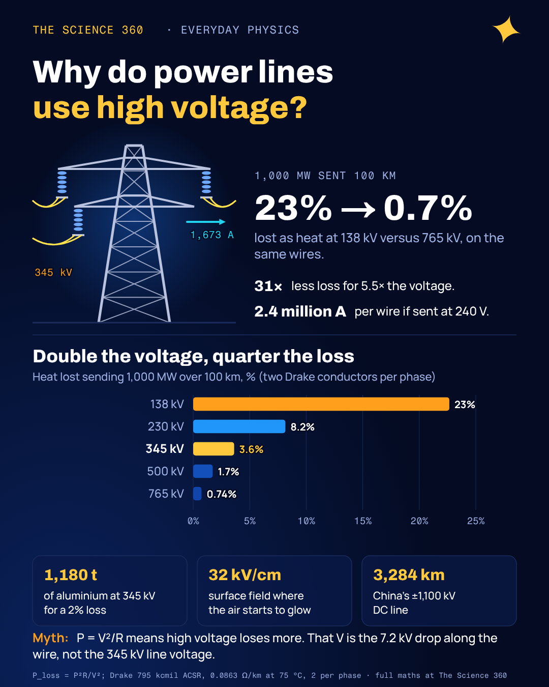
If you tried to send the output of one big power station, 1,000 megawatts, down a three-phase line at the 240 volts in your house, each wire would have to carry about 2.4 million amps. No cable on Earth carries that. Step the same power up to 345,000 volts and the current falls to about 1,700 amps, which a pair of ordinary aluminium conductors the thickness of your thumb handles all day.

Everyone knows the one-line reason: higher voltage, lower current, less heat. What the usual explanations skip is how big the effect is on a real line, why the industry stopped climbing at around a million volts, and why the longest lines in the world are not AC at all. We will do all three with numbers from an actual conductor datasheet.

Quick answerFor a fixed power, current falls as voltage rises (

P = VI

), and wire heating rises with current squared (

P_{\mathrm{loss}} = I^2R

). So doubling the voltage cuts losses to a quarter. Sending 1,000 MW 100 km loses about 23% at 138 kV but only 0.7% at 765 kV on the same wire.

Infographic: Why do power lines use high voltage? A lattice transmission tower carries three phases, each a pair of conductors, with 1,673 amps flowing at 345 kV. Sending 1,000 MW over 100 km on the same wires loses 23% as heat at 138 kV but only 0.7% at 765 kV, 31 times less for 5.5 times the voltage. A bar chart shows loss falling as one over voltage squared: 23% at 138 kV, 8.2% at 230 kV, 3.6% at 345 kV, 1.7% at 500 kV and 0.74% at 765 kV. Holding loss to 2% at 345 kV takes about 1,180 tonnes of aluminium. — Tap the image to view it full size. View the accessible, editable SVG.

Why does high voltage reduce power loss?

Two equations do all the work. The power a line delivers is voltage times current. The power it wastes heating its own conductors is current squared times their resistance. Fix the power you need to deliver, and the current is set by the voltage you choose:

\begin{aligned}I &= \frac{P}{\sqrt{3}\, V_{LL}} \\ P_{\mathrm{loss}} &= 3 I^2 R_{\mathrm{phase}} = \frac{P^2 R_{\mathrm{phase}}}{V_{LL}^2}\end{aligned}

This is for a three-phase line at unity power factor. Loss scales as $1/V^2$ .

The square is the whole story. Doubling the voltage halves the current, and because the loss depends on current squared, it falls to a quarter. Going from 138 kV to 765 kV, a factor of 5.5 in voltage, cuts the loss by a factor of 31.

A worked example on a real conductor

Take one of the most common transmission conductors in North America, 795 kcmil "Drake" ACSR (aluminium strands around a steel core). Its datasheet gives an AC resistance of 0.0263 Ω per 1,000 ft at 75 °C, which is 0.0863 Ω/km, an outside diameter of 1.108 inches and a rated current of 907 A. Use two of them per phase, a common arrangement at 345 kV, and send 1,000 MW down a 100 km line.

Step 1. Current per phase at 345 kV

I = \frac{1{,}000\times10^{6}\ \mathrm{W}}{1.732 \times 345{,}000\ \mathrm{V}} = \mathbf{1{,}673\ A}

That is 837 A in each conductor, under the 907 A rating.

Step 2. Resistance per phase

R = \frac{0.0863\ \Omega/\mathrm{km} \times 100\ \mathrm{km}}{2\ \text{conductors}} = \mathbf{4.31\ \Omega}

Step 3. Heat lost

\begin{aligned}P_{\mathrm{loss}} &= 3 \times 1{,}673^2 \times 4.31 \\ &= 3 \times 2.80\times10^{6} \times 4.31 \\ &= \mathbf{36\ MW}\ (3.6\%)\end{aligned}

Same conductors, other voltages

138 kV: I = 4,184 A, loss = 227 MW (23%), and 2,092 A per conductor, far above the rating. 765 kV: I = 755 A, loss = 7.4 MW (0.74%).

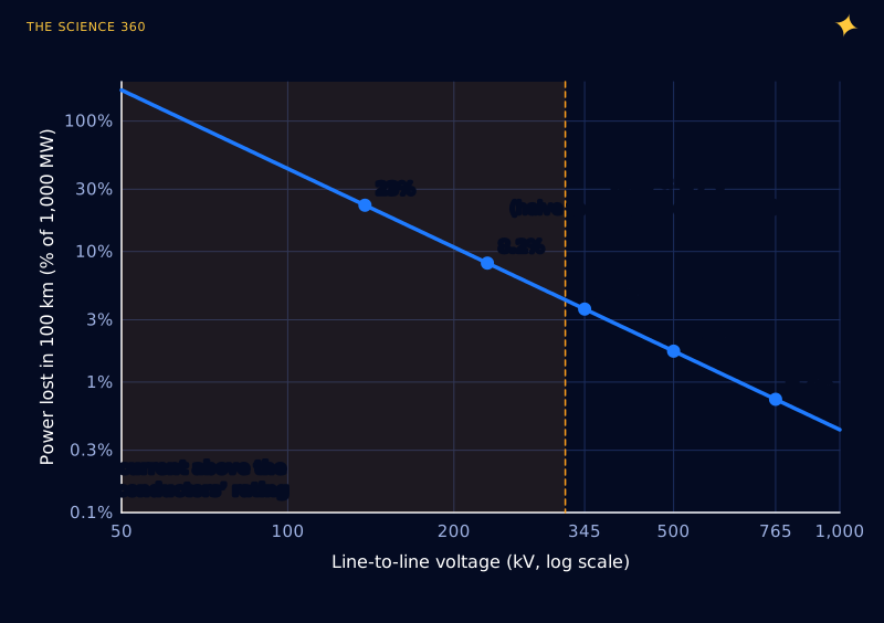
Figure 1. Loss for 1,000 MW over 100 km on a two-conductor Drake bundle per phase, computed from the datasheet resistance at 75 °C. Left of the dashed line the conductors could not carry the current at all without overheating. The slope of minus two on log axes is the 1/V² law.

Figure 1 shows the second, less obvious point. At low voltage, wasted energy is the smaller problem. The current would melt the line. The 138 kV case asks each conductor for 2,092 A, more than twice its thermal rating. At low voltage you do not get a lossy line; you get no line, unless you add a lot more metal.

The misconception: “P = V²/R means high voltage loses more”

Students meet three versions of the power formula ( $P = VI$ , $P = I^2R$ and $P = V^2/R$ ) and reasonably ask: if loss is $V^2/R$ , shouldn't higher voltage mean more loss? The formula is right. The $V$ is the wrong voltage.

In $P = V^2/R$ applied to the wire, $V$ is the voltage dropped along the conductor, from one end to the other, not the line's voltage to ground. Check it with the 345 kV example:

\begin{aligned}\Delta V &= IR = 1{,}673\ \mathrm{A} \times 4.31\ \Omega = 7.2\ \mathrm{kV} \\ P_{\mathrm{loss}} &= \frac{3 \times (7{,}220\ \mathrm{V})^2}{4.31\ \Omega} = \mathbf{36\ MW} \\ V_{\mathrm{phase}} &= \frac{345\ \mathrm{kV}}{\sqrt{3}} = 199\ \mathrm{kV} \\ \frac{\Delta V}{V_{\mathrm{phase}}} &= \frac{7.2}{199} = 3.6\%\end{aligned}

The $V^2/R$ form gives the same answer, once $V$ is the drop along each phase.

The 199 kV between the wire and the ground never drives current through the wire's resistance. It sits across the load at the far end, which is where you want your power to go. Raising the transmission voltage lowers the current, which lowers the drop along the wire, which lowers the loss. All three formulas agree once you put the right voltage in each.

A second, quieter misconception: that high voltage is needed to "push" electricity a long way. Voltage is not a push that runs out over distance. A 12 V car battery would deliver power through 1,000 km of wire just fine if the wire were thick enough. The question is only how much conductor you are willing to buy.

How much metal does high voltage save?

That second framing is how utilities actually think. Fix an acceptable loss, say 2%, and ask how much aluminium the line needs. Because the allowed resistance scales with $V^2$ , the cross-section, and therefore the mass of metal, scales as $1/V^2$ .

Aluminium for 1,000 MW, 100 km, 2% loss, at 345 kV

\begin{aligned}P_{\mathrm{loss}} &= 0.02 \times 1{,}000\ \mathrm{MW} = 20\ \mathrm{MW} \\ R &= \frac{20\times10^{6}}{3 \times 1{,}673^2} = 2.38\ \Omega \\ A &= \frac{\rho L}{R} = \frac{3.48\times10^{-8} \times 100{,}000}{2.38} \\ &= 1.46\times10^{-3}\ \mathrm{m^2}\ (1{,}460\ \mathrm{mm^2}) \\ m &= 3 \times 1.46\times10^{-3} \times 100{,}000 \times 2{,}700 \\ &= \mathbf{1{,}180\ tonnes}\end{aligned}

$\rho$ here is the effective resistivity implied by Drake's datasheet resistance and 403 mm² of aluminium; the mass covers all three phases.

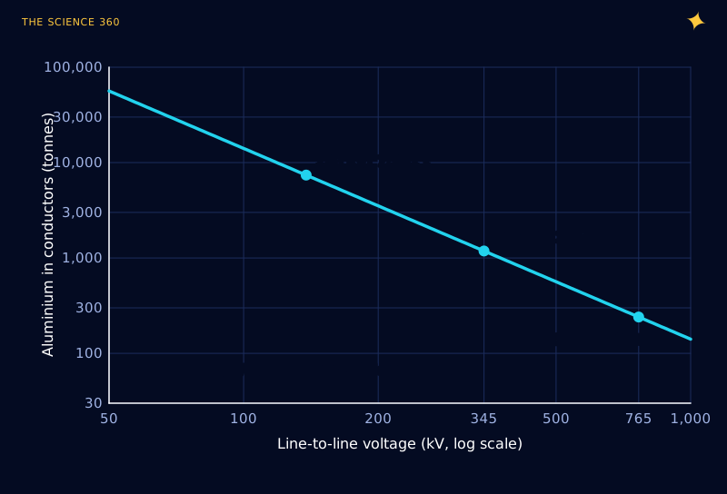
Log-log plot of tonnes of aluminium needed against line voltage for 1000 megawatts over 100 kilometres with 2 percent loss. The line falls from about 50,000 tonnes at 50 kV to 7,391 tonnes at 138 kV, 1,183 tonnes at 345 kV and 241 tonnes at 765 kV. — Figure 2. Conductor aluminium needed to hold losses to 2%, computed from the Drake datasheet resistance. Every doubling of voltage saves three quarters of the metal, and the towers that hold it up get lighter too.

At 138 kV you would need over 7,000 tonnes of aluminium per 100 km; at 765 kV, about 240. That factor of 31 in metal, and in the steel towers needed to hold it up, is the economic reason transmission voltages climbed through the twentieth century, from tens of kilovolts to 345, 500 and 765 kV in North America and 400 kV across much of Europe.

Why not use even higher voltage?

If $1/V^2$ is so generous, why stop at 765 kV? Several costs grow with voltage, and the first one you hit is visible at night as a faint violet glow.

Corona: the air around the wire breaks down

Air ionises when the electric field exceeds roughly 30 kV/cm. A transmission conductor is a thin cylinder, and the field at its surface is concentrated by its small radius. When the surface field passes the onset value, the air right around the wire glows, hisses and crackles. This is corona, and it wastes power, makes audible noise and causes radio interference, all worse in rain.

Peek's law gives the onset field for a cylindrical conductor. For Drake (radius 1.41 cm), with a surface factor of 0.85 for a stranded, weathered cable in air at standard density:

\begin{aligned}E_{\mathrm{onset}} &= 30\, m\, \delta \left(1 + \frac{0.301}{\sqrt{\delta r}}\right)\ \mathrm{kV/cm} \\ &= 30 \times 0.85 \times 1 \times \left(1 + \frac{0.301}{\sqrt{1.41}}\right) \\ &= 30 \times 0.85 \times 1.254 = \mathbf{32\ kV/cm}\end{aligned}

That onset field is a peak value. Surface field of a single conductor, phase-to-ground peak voltage $V_p$ , phase spacing $D$ :

E = \frac{V_p}{r \ln(D/r)}

At 345 kV, with $D \approx 7.5$ m:

\begin{aligned}V_p &= \frac{345 \times \sqrt{2}}{\sqrt{3}} = 282\ \mathrm{kV} \\ E &= \frac{282}{1.41 \times \ln(750/1.41)} \\ &= \frac{282}{1.41 \times 6.28} = \mathbf{32\ kV/cm}\end{aligned}

A single Drake conductor at 345 kV sits right at corona onset. That is why 345 kV lines in practice use two conductors per phase, and 765 kV lines use four or six. Splitting the phase into a bundle spaced about 45 cm apart makes it look electrically like a much fatter conductor, which lowers the surface field.

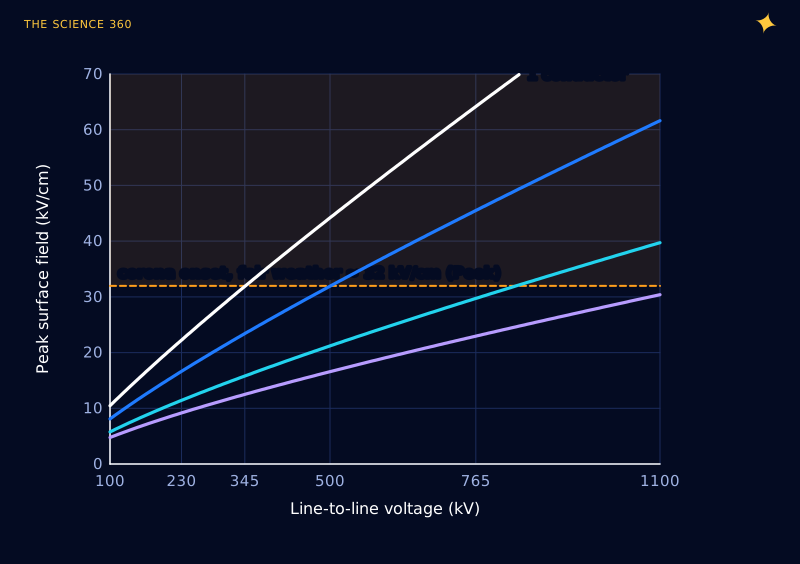
Plot of peak conductor surface field against line voltage from 100 to 1100 kV for 1, 2, 4 and 6 Drake sub-conductors per phase. The single conductor crosses the corona onset of about 32 kilovolts per centimetre near 345 kV, the 2-bundle near 500 kV, the 4-bundle near 830 kV, and the 6-bundle stays just below it at 1100 kV. — Figure 3. Peak surface field versus voltage for bundles of Drake conductors (45.7 cm sub-conductor spacing, phase spacing assumed to grow from about 4 m at 138 kV to 14 m at 765 kV). Above the dashed line the air around the wire ionises. Designers keep well below it because rain, insects and surface damage lower the real onset.

Each extra sub-conductor means more weight, more hardware and stronger towers, so the corona limit acts as a steadily rising cost per kilovolt rather than a hard wall.

Clearances, insulators and surges

The air gaps from conductor to tower and to the ground must withstand the operating voltage plus the brief surges from switching and lightning, which can reach a few times normal. Insulator strings at 765 kV are several metres long, tower heads are wide enough to park a truck in, and rights of way get broader. Transformers and circuit breakers for the highest voltages are enormous; the converter transformers built for China's ±1,100 kV DC line weigh about 800 tonnes each.

Together these set a practical ceiling around 1,000 to 1,100 kV. China operates 1,000 kV AC lines, and the ±1,100 kV Changji to Guquan DC link carries 12 GW over 3,284 km from Xinjiang to Anhui. That is about where everyone has stopped, at least for now.

Why the longest lines are DC

An AC line is more than a resistor. It has series inductance and capacitance to ground spread along its whole length, and those set two limits that DC does not have.

The first is charging current. Every kilometre of line or cable is a capacitor that must be charged and discharged 50 or 60 times a second. On underground and undersea cables, where the capacitance is large, the charging current can use up the conductor's whole rating within a few tens of kilometres, leaving no room for useful power.

The second is stability. Power flows over an AC line because the voltage at the sending end leads the receiving end in phase. For a lossless line, the transfer is:

P = \frac{V_S V_R}{Z_c} \cdot \frac{\sin\delta}{\sin(\beta l)}

$V^2/Z_c$ is the surge impedance loading (SIL). For a 765 kV line with $Z_c \approx 260\ \Omega$ :

\mathrm{SIL} = \frac{765^2}{260} = \mathbf{2{,}250\ MW}

$\beta = 2\pi/\lambda$ , with $\lambda \approx 5{,}000$ km at 60 Hz. At a safe angle $\delta = 30^\circ$ :

\begin{aligned}300\ \mathrm{km}:\ \frac{P}{\mathrm{SIL}} &= \frac{0.5}{\sin 21.6^\circ} = \mathbf{1.36} \\ 800\ \mathrm{km}:\ \frac{P}{\mathrm{SIL}} &= \frac{0.5}{\sin 57.6^\circ} = \mathbf{0.59}\end{aligned}

Figure 4. Why long AC lines carry less: the stability limit from the lossless-line equation at a 30° angle, compared with the empirical St Clair curve that utilities use. The thermal cap at 3 × SIL is illustrative. DC has no phase angle, so it can run at its thermal limit regardless of length.

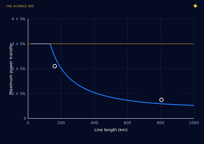
The simple formula lands close to the industry's empirical St Clair curve, which reads about 2.1 × SIL at 100 miles and 0.75 × SIL at 500 miles. Long AC lines can be helped with series capacitors and other compensation, but the trend is unavoidable. DC has no phase angle and no charging current once the line is energised, so a DC line can run near its thermal limit at any length.

DC also loses less per kilometre. The usual comparison quotes about 3.5% per 1,000 km for HVDC against about 6.7% for AC at the same voltage, partly because DC has no skin effect and roughly half the corona loss for the same power. What DC pays for is the converter stations at each end, which are expensive and lossy in their own right. The break-even is commonly put at about 600 to 800 km for overhead lines and about 50 km for submarine cables, which is why nearly every long undersea interconnector is DC.

How much electricity is lost on the way to you?

The US Energy Information Administration estimates that transmission and distribution losses averaged about 5% of electricity in the United States from 2018 through 2022. The $1/V^2$ law tells you where to look for it: the high-voltage backbone loses relatively little per kilometre, while a large share of the losses typically occurs in the lower-voltage distribution network and transformers near the customer, where currents are higher. That is why the final step down to 240 V or 120 V happens on a pole or pad-mounted transformer just a few houses away, so the low-voltage, high-current part of the trip is as short as possible.

The rule of thumb: for the same wire and the same power, loss scales as 1/V². Doubling the voltage quarters the loss, or lets you use a quarter of the metal. The limits on going higher are air (corona), insulation and the size of transformers, and for long distances the limits of AC itself, which is where HVDC takes over.

FAQ

Why does high voltage reduce power loss?

For a given power, current is power divided by voltage, and the heat lost in the wire is current squared times resistance. Doubling the voltage halves the current and cuts the loss to a quarter. In a worked example, sending 1,000 MW over 100 km loses about 23% at 138 kV, 3.6% at 345 kV and 0.7% at 765 kV on the same conductors.

Doesn’t P = V squared over R mean higher voltage gives more loss?

No. In that formula V is the voltage dropped along the wire itself, not the line's voltage to ground. Raising the transmission voltage lowers the current, which lowers the voltage drop along the wire, so the loss falls.

Why not use even higher voltages?

Above a few hundred kilovolts the electric field at the conductor surface starts to ionise the air (corona), wasting power and making noise, so lines need bundles of several conductors per phase. Clearances, insulator strings, towers and transformers also grow with voltage. The highest in service is China's plus or minus 1,100 kV DC Changji to Guquan line.

How much electricity is lost in transmission and distribution?

The US Energy Information Administration estimates about 5% of electricity transmitted and distributed in the United States was lost in 2018 through 2022.

When is HVDC better than AC?

For long distances and undersea cables. HVDC avoids the reactive charging current and stability limits of long AC lines, and loses roughly 3.5% per 1,000 km against about 6.7% for AC. The converter stations are expensive, so the break-even is about 600 to 800 km overhead and about 50 km for submarine cables.

Sources

795 kcmil Drake ACSR specifications (AC resistance 0.026 Ω/1,000 ft at 75 °C, diameter 1.108 in, 907 A): nassaunationalcable.com/products/795-d-acsr
US Energy Information Administration, "How much electricity is lost in electricity transmission and distribution in the United States?" (about 5%, 2018 to 2022): eia.gov/tools/faqs/faq.php?id=105
Wikipedia, "Peek's law" (corona onset gradient, air density and surface factors): en.wikipedia.org/wiki/Peek's_law
Wikipedia, "High-voltage direct current" (break-even distances, 3.5% versus 6.7% per 1,000 km, corona and charging current): en.wikipedia.org/wiki/High-voltage_direct_current
eeNews Europe, record 1,100 kV UHVDC link in China (12 GW, 3,284 km): eenewseurope.com
T&D World, first 1,100 kV UHVDC link uses ABB transformers (800 tonnes each): tdworld.com
Line loadability and the St Clair curve (SIL of a 765 kV line about 2,247 MW; 2.1 × SIL at 100 miles, 0.75 × SIL at 500 miles), worked example: electricalbaba.com; background: WRLDC, "Line Loadability in Indian Perspective": posoco.in (PDF)

Method note: loss figures assume unity power factor, a flat 75 °C conductor temperature and no line charging; phase spacings in Figure 3 are typical values I assumed, not a specific line's design. Real lines carry varying loads, so annual energy losses are lower than the full-load percentages above.

Header image: NASA (image iss073e0685684), regraded for this article.

Why does high voltage reduce power loss?

A worked example on a real conductor

The misconception: “P = V²/R means high voltage loses more”

How much metal does high voltage save?

Why not use even higher voltage?

Corona: the air around the wire breaks down

Clearances, insulators and surges

Why the longest lines are DC

How much electricity is lost on the way to you?

FAQ

Why does high voltage reduce power loss?

Doesn’t P = V squared over R mean higher voltage gives more loss?

Why not use even higher voltages?

How much electricity is lost in transmission and distribution?

When is HVDC better than AC?

Related on The Science 360

Sources