Why 100nF Decoupling Capacitors? The Impedance Math • The Science 360

Quick answer 100 nF is a habit from 1970s TTL design, when it was the largest practical low-inductance ceramic. On a modern board it works best near 10 to 25 MHz. Above that, ESL plus about 1 nH of via loop set the impedance, so placement matters more than value, and 1 µF in the same package is often better.

Infographic: Why is every bypass capacitor 100 nF? A board cross-section shows a capacitor beside a chip and the via loop down to the power planes. Once mounted, a 100 nF and a 1 µF 0402 both measure about 0.93 to 0.94 ohms at 100 MHz, because 1.5 nH of loop inductance sets the impedance. A log chart of impedance against frequency shows the 100 nF notch moving from 25 MHz bare to 13 MHz mounted, and the 1 µF part ten times lower below 25 MHz before joining the same inductive line. Tiles: a pulse droops the capacitor by 10 mV but the loop by 150 mV, and a 4.7 µF 0805 keeps 33% at 12 V. — Tap the image to view it full size. View the accessible, editable SVG.

Open almost any reference schematic and you will find the same part next to every power pin: a 100 nF ceramic, written 0.1 µF or "104". It may be the most copied number in electronics, and most people who place it could not tell you why it is 100 nF and not 47 nF or 1 µF.

In January 2025 Hackaday ran a piece with the blunt title "Capacitor Decoupling Chaos, And Why You Should Abandon 100 nF", summarising a long analysis by Graham Sutherland. The conclusion was that the decoupling effect of a lone 100 nF is "pretty miserable" and that a 1 µF ceramic usually does better. The comments split into two camps. So let us build the impedance curves from real parasitic values, include the PCB vias, and see where 100 nF wins and where it loses.

What does a decoupling capacitor actually do?

A digital chip does not draw a steady current. On every clock edge thousands of transistors switch at once and pull a spike of charge for a nanosecond or two. The regulator is centimetres away, behind tens of nanohenries of trace inductance, and it reacts in microseconds. Without a local reservoir the supply pin sags.

The decoupling capacitor is that local reservoir. The useful way to judge one is not "how much charge does it hold" but "what impedance does it present between the power pin and ground at the frequencies where the chip is drawing current". A common target follows straight from Ohm's law: allowed ripple divided by the current step.

Target impedance for a 3.3 V rail, 3% allowed ripple, 1 A current step:

\begin{aligned}\Delta V_{\mathrm{allowed}} &= 3.3 \times 0.03 = 0.099\ \mathrm{V} \\ Z_{\mathrm{target}} &= \Delta V/\Delta I = 0.099/1 \\ &\approx \mathbf{0.1\ \Omega}\end{aligned}

The decoupling network must stay below about 0.1 Ω across the band where the chip draws current.

Here is the first misconception. People picture the capacitor as a bucket that runs dry if it is too small. Run the numbers and the bucket is almost never the problem.

Charge drawn by a 100 mA pulse lasting 10 ns, and the droop of a 100 nF capacitor supplying it:

\begin{aligned}Q &= It = 0.1 \times 10 \times 10^{-9} = 1\ \mathrm{nC} \\ \Delta V &= Q/C = 1\ \mathrm{nC}/100\ \mathrm{nF} = \mathbf{10\ mV}\end{aligned}

Voltage across 1.5 nH of loop inductance if that current ramps in 1 ns:

\begin{aligned}V &= L\,\frac{di}{dt} = 1.5{\times}10^{-9} \times \frac{0.1}{10^{-9}} \\ &= \mathbf{150\ mV}\end{aligned}

The inductance in the path costs fifteen times more voltage than the capacitance does. That single comparison explains most of what follows.

A real capacitor is an R, an L and a C in series

Every multilayer ceramic capacitor (MLCC) has three things in series: the capacitance C, a small equivalent series resistance (ESR) from the electrodes and terminations, and an equivalent series inductance (ESL) from the current loop through the part. The impedance magnitude is

|Z| = \sqrt{\mathrm{ESR}^2 + \left(2\pi f\,\mathrm{ESL} - \frac{1}{2\pi f C}\right)^2}

At low frequency the 1/(2πfC) term dominates and impedance falls at 20 dB per decade. At high frequency 2πf·ESL wins and impedance rises at 20 dB per decade, like an inductor. Where the reactances cancel, impedance bottoms out at the ESR: the self-resonant frequency (SRF).

How big is ESL? In a classic AVX study, Jeffrey Cain measured 0.1 µF MLCCs and found 870 pH for 0603, 1050 pH for 0805 and 1200 pH for 1206, with sample spread within about ±7%. He also found that inside one package the inductance barely changes with capacitance value: a 0.01 µF and a 1 µF 1206 had the same high-frequency impedance line within ±10%. TDK's current equivalent-circuit model for its general 0402 series uses 0.28 nH. We will use 0.4 nH for 0402 (a middle-of-the-road value) and Cain's 0.87 nH for 0603. The ESR values in the plots (5 to 60 mΩ) are representative of X7R and X5R parts at resonance; your datasheet curve will differ somewhat.

Worked example: self-resonant frequency of a bare 100 nF 0402.

\begin{aligned}f_{\mathrm{SRF}} &= \frac{1}{2\pi\sqrt{LC}} \\ LC &= 0.4{\times}10^{-9} \times 100{\times}10^{-9} \\ &= 4.0 \times 10^{-17}\ \mathrm{s^2} \\ \sqrt{LC} &= 6.32 \times 10^{-9}\ \mathrm{s} \\ 2\pi\sqrt{LC} &= 3.97 \times 10^{-8}\ \mathrm{s} \\ f_{\mathrm{SRF}} &\approx \mathbf{25\ MHz}\end{aligned}

Same part in 0603 (0.87 nH):

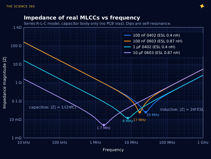
\begin{aligned}\sqrt{0.87{\times}10^{-9} \times 10^{-7}} &= 9.33 \times 10^{-9}\ \mathrm{s} \\ f_{\mathrm{SRF}} &\approx \mathbf{17\ MHz}\end{aligned}

Log-log plot of impedance versus frequency for four ceramic capacitors: 100 nF 0402 resonates at 25 MHz, 100 nF 0603 at 17 MHz, 1 µF 0402 at 8 MHz and 10 µF 0603 at 1.7 MHz; curves with equal ESL merge above resonance. — Figure 1. Computed |Z| of four MLCCs (capacitor body only). Notice that the 1 µF 0402 (green) and the 100 nF 0402 (blue) sit on the same inductive line above 30 MHz, because they share a package and therefore an ESL.

Figure 1 already holds the punchline. Below 25 MHz the green 1 µF is up to ten times lower in impedance than the blue 100 nF. Above about 30 MHz they land on the same line. Swapping 100 nF for 1 µF in the same package costs nothing at high frequency and buys a decade at low frequency. That is the core of the Hackaday argument, and for the bare part it is right.

Why the vias matter more than the capacitor

A capacitor on a datasheet is not a capacitor on a board. Current has to leave the IC pin, run along a trace or pad, drop through a via to the power plane, cross the plane, come up another via, through the capacitor, and back. That loop has inductance, usually more than the capacitor itself.

How much? All About Circuits puts a conventional side-by-side via pair at about 1.1 nH, falling to about 0.7 nH with the vias tucked close together. Cadence works a via pair example at 1.53 nH, already more than the capacitor's ESL. LearnEMC's measured examples run from 0.61 nH for a very tight pad design to about 16 nH with an inch of trace in the path.

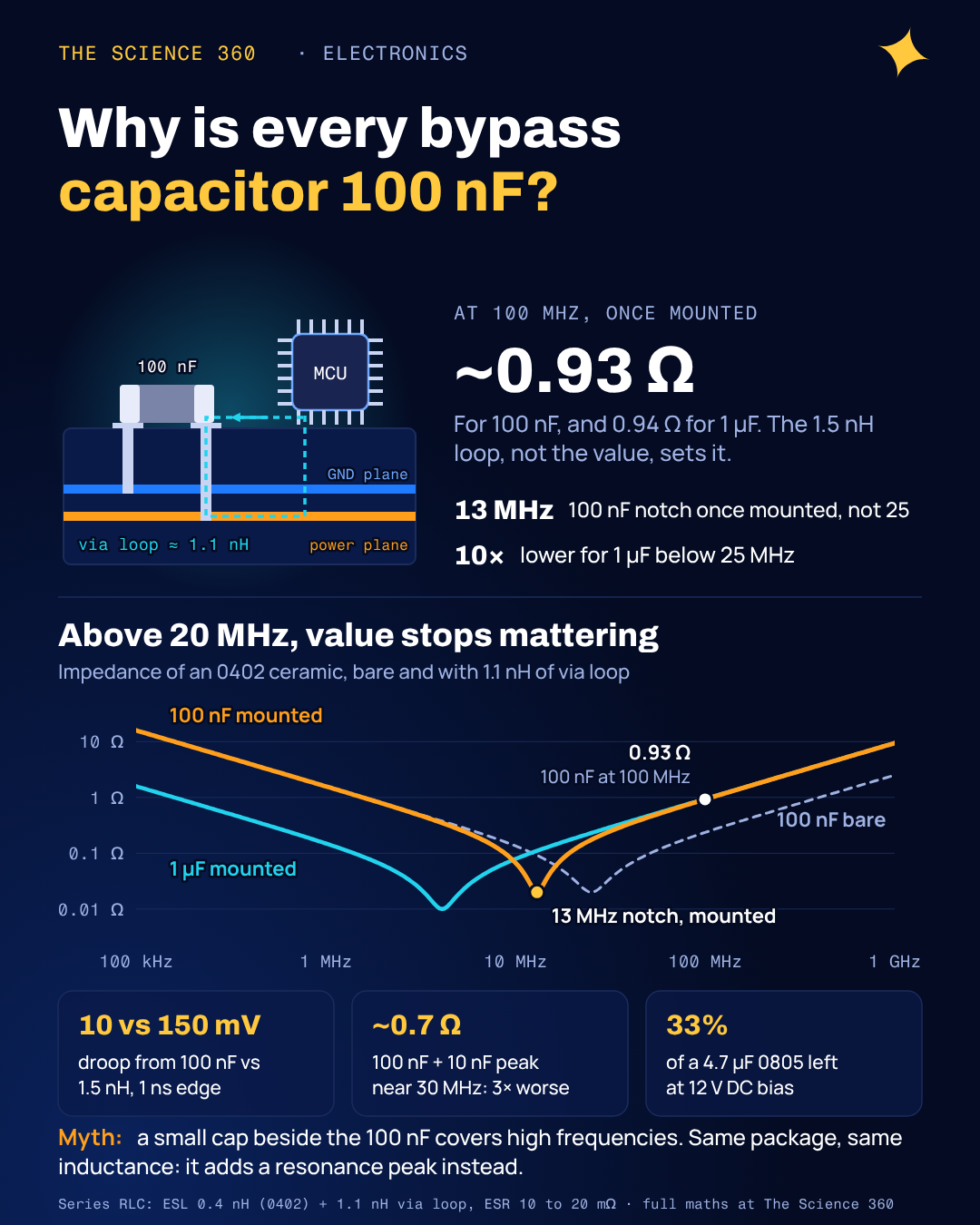
So add 1.1 nH of mounting inductance to every part in Figure 1 and redraw.

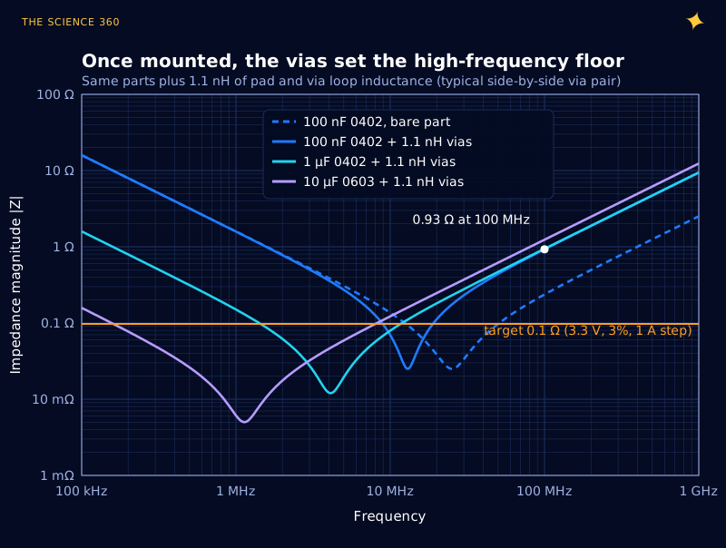
Impedance versus frequency for 100 nF, 1 µF and 10 µF capacitors each with 1.1 nH of via inductance; above about 20 MHz all three curves merge into one inductive line, so the capacitor value no longer matters. — Figure 2. The same capacitors with 1.1 nH of via loop added. The dashed curve is the bare 100 nF from Figure 1. Above roughly 20 MHz every curve is set by inductance alone, and none of them meets a 0.1 Ω target.

Worked example: the same 100 nF 0402 once mounted, with 1.1 nH of vias and pads.

\begin{aligned}L_{\mathrm{total}} &= 0.4 + 1.1 = 1.5\ \mathrm{nH} \\ f_{\mathrm{SRF}} &= \frac{1}{2\pi\sqrt{1.5{\times}10^{-9} \times 10^{-7}}} \\ &= \frac{1}{2\pi \times 1.22 \times 10^{-8}} \approx \mathbf{13\ MHz}\end{aligned}

At 100 MHz:

\begin{aligned}X_L &= 2\pi \times 10^8 \times 1.5{\times}10^{-9} = 0.94\ \Omega \\ X_C &= \frac{1}{2\pi \times 10^8 \times 10^{-7}} = 0.016\ \Omega \\ |Z| &\approx 0.94 - 0.016 \approx \mathbf{0.93\ \Omega}\end{aligned}

The capacitance contributes under 2%. For 1 µF in the same footprint, X_C = 0.0016 Ω and |Z| ≈ 0.94 Ω. Identical, to the eye.

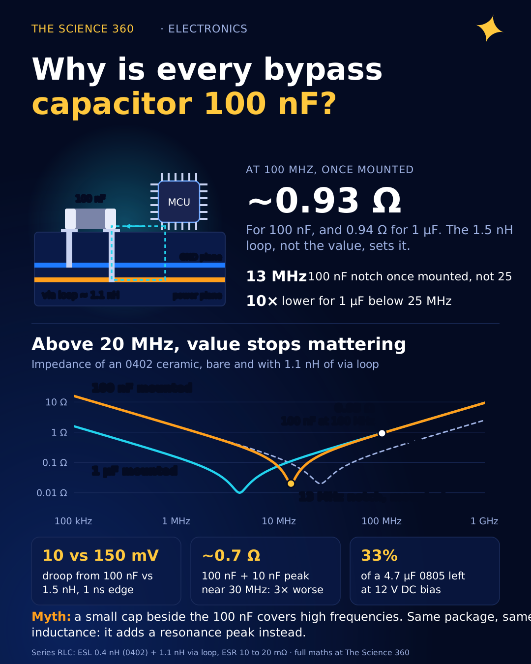
Three things fall out of Figure 2. First, the SRF of the 100 nF dropped from 25 MHz to 13 MHz, and the curve above it moved up almost fourfold. The part did not change. The board did.

Second, against our 0.1 Ω target, a single mounted 100 nF only qualifies between about 9 and 19 MHz. A single mounted 1 µF qualifies from about 1.4 to 12 MHz. A 10 µF 0603 covers 0.16 to 8 MHz. None of them covers 100 MHz, where a single mounted capacitor of any value sits near 1 Ω. Up there you rely on many capacitors in parallel (each identical one divides the inductance), short via loops, plane capacitance and the chip's on-die capacitance.

Third, and this answers the title, the value of a small MLCC mostly decides where its notch lands. The package and the layout decide how good it is above the notch. 100 nF puts the notch around 10 to 25 MHz, a sensible place when TTL had edges of several nanoseconds. For a modern MCU clocked anywhere from 16 to 200 MHz, the notch is not magic. It is just somewhere.

Where did 100 nF come from?

The honest answer is that nobody wrote it down as a rule with a derivation. What we can document is that 1970s TTL guidance already used this range. A reproduction of a 1970s TTL system design guide (the Sams "Guide to Transistor-Transistor Logic" series) says to "decouple every 5 to 10 packages with rf capacitors of 0.01 to 0.1 µF" and to put 0.1 µF at the Vcc pins of line drivers and receivers. Analog Devices' MT-101 tutorial, much later, still puts the high-frequency bypass at 0.01 to 0.1 µF with a 10 to 100 µF electrolytic nearby.

Hackaday commenters offer the usual explanation: 0.1 µF was about the largest ceramic you could buy cheaply, and its resonance sat above what the logic of the day generated. Treat that as plausible folklore, not settled history. What is not folklore is that a modern 0402 holds 1 µF or more with the same ESL as the old 100 nF, which removes the original reason to stop at 0.1 µF.

Is the 100 nF + 10 nF combination a good idea?

The next layer of folk wisdom says to put a smaller capacitor next to the 100 nF, say 10 nF or 1 nF, "to cover the higher frequencies". This is the misconception that does the most damage, because the intuition is half right and the result can be worse than doing nothing.

If both capacitors share the same package and roughly the same via loop, they share the same inductance, so above both resonances they behave identically. The smaller one cannot be "better at high frequency". Between the two SRFs, though, the 100 nF has already turned inductive while the 10 nF is still capacitive. An inductor in parallel with a capacitor is a tank circuit, and a tank circuit has a parallel resonance where impedance spikes.

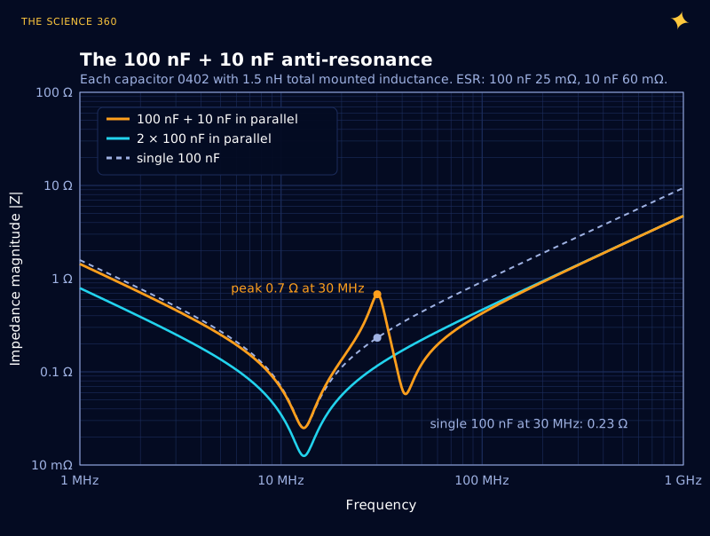
Impedance of 100 nF and 10 nF capacitors in parallel shows an anti-resonance peak of about 0.7 ohm near 30 MHz, three times higher than a single 100 nF at that frequency, while two equal 100 nF capacitors give a smooth curve. — Figure 3. A 100 nF and a 10 nF in parallel, each with 1.5 nH total mounted inductance. The anti-resonance near 30 MHz reaches about 0.7 Ω. A single 100 nF alone is 0.23 Ω there, and two 100 nF in parallel are 0.12 Ω.

In this model the pair hits about 0.68 Ω at 30 MHz. A lone 100 nF is 0.23 Ω at the same frequency, so adding the 10 nF made that band three times worse. Two identical 100 nF capacitors give 0.12 Ω there with no peak at all. The height of the peak depends on the ESR: higher ESR damps it, which is one reason ultra-low-ESR C0G parts in a decoupling array can be a bad idea. In Compliance Magazine's rule of thumb is to parallel equal values, or values no more than a decade apart, and to damp any resonance between sections with a ferrite or a small resistor.

How the via geometry sets the inductance

The loop inductance of two parallel vias is close to the classic two-wire formula. Cadence gives it as $L \approx 0.4\,h\,[\ln(2s/d) + 0.25]\ \mathrm{nH}$ , where h is the depth from the capacitor to the plane pair in millimetres, s is the via centre spacing and d the via diameter. The ln term grows slowly, so spacing helps, but h appears as a straight multiplier.

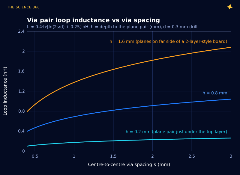
Line chart of via pair loop inductance against via spacing for three plane depths: at 1.6 mm depth the loop is about 0.9 to 2.1 nH, at 0.8 mm about 0.5 to 1.0 nH, and at 0.2 mm depth it stays below 0.3 nH. — Figure 4. Via pair loop inductance from the two-wire formula. Halving the via spacing from 2 mm to 1 mm saves about 25%. Moving the plane pair from 1.6 mm to 0.2 mm below the capacitor saves about 88%.

Worked example: via pair, 0.3 mm drill, 1 mm apart, planes 1.6 mm down.

\begin{aligned}\ln(2s/d) &= \ln(2 \times 1.0/0.3) = \ln 6.67 \\ &= 1.90 \\ L &\approx 0.4 \times 1.6 \times (1.90 + 0.25) \\ &= \mathbf{1.37\ nH}\end{aligned}

Same vias, planes 0.2 mm down (thin core under the top layer):

L \approx 0.4 \times 0.2 \times 2.15 = \mathbf{0.17\ nH}

That 1.37 nH is more than three times the ESL of the 0402 capacitor. This is why stack-up choice (a thin dielectric between the top layer and the first ground and power planes) does more for high-frequency decoupling than any choice of capacitor value.

The DC bias trap: your 10 µF may be 3 µF

If you take the advice to go bigger, there is a catch. Class II ceramics like X5R and X7R lose capacitance as DC voltage is applied, and small packages lose the most. Mark Fortunato's Maxim (now Analog Devices) tutorial on this has the memorable title "Why Your 4.7 µF Capacitor Becomes a 0.33 µF Capacitor". In his comparison of 4.7 µF X7R parts at 12 V bias, an 0805 kept about 33% of its rated value, a 1206 about 73%, and a 1210 about 89%. He also found that the voltage rating within a given package told you surprisingly little, and that "X7R" says nothing about voltage coefficient at all.

Low-value parts generally suffer less, but for a 10 µF 0603 on a 5 V rail, losing half or more is routine. Open the manufacturer's DC bias curve for the exact part number and design with the derated value. For decoupling, lost capacitance only shifts the notch up in frequency. The inductive side of the curve does not move.

Practical rules for placing decoupling capacitors

Putting the numbers together, here is what we would actually do on a new board:

Start from the IC datasheet. The manufacturer knows about on-die capacitance that you do not.
Use the largest value that is cheap in your smallest practical package. In 0402, 1 µF is usually a better default than 100 nF. Check DC bias at your rail voltage and any inrush limit on the regulator.
Fight inductance, not capacitance. Vias in or right at the pads, power and ground vias close together, no trace between pad and via, capacitor on the side nearest the planes (Clemson's EMC lab gives the same rules).
Choose the stack-up for decoupling. A plane 0.1 to 0.2 mm under the component layer beats any capacitor value.
Parallel equal values rather than staggered 100n plus 10n in the same footprint. If you must mix, simulate the PDN or add damping.
Keep a bulk capacitor (10 to 100 µF) per rail near the regulator to cover the low-kHz to MHz range where the regulator loop runs out of bandwidth.

Capacitor ESR and ESL return at much larger currents in our how a buck converter works walkthrough, and impedance as the real figure of merit is the whole story of why coax is 50 ohms.

So should you abandon 100 nF?

Abandon it as a reflex, not as a part. A well-placed 100 nF next to a slow microcontroller works fine, and millions of products prove it. But above a few tens of MHz the 1 to 2 nH of via loop sets the impedance, and a 100 nF and a 1 µF in the same footprint are indistinguishable there. Below that, the bigger part wins. If you change one habit, make it this: look at the vias before you look at the value.

FAQ

Why are decoupling capacitors usually 100 nF?

Mostly habit inherited from 1970s TTL design, when 0.01 to 0.1 µF was the largest practical low-inductance ceramic and logic edges were slow. A modern 100 nF MLCC still works because its impedance is low from a few MHz up to a few tens of MHz, but above about 20 MHz the mounting inductance, not the capacitance, sets the impedance.

Can I use a 1 µF capacitor instead of 100 nF for decoupling?

Usually yes, and it is often better. In the same 0402 or 0603 package a 1 µF MLCC has roughly the same ESL as a 100 nF part, so it matches the 100 nF above resonance and beats it by ten times below resonance. Check the IC datasheet, inrush limits and the DC bias derating of the part you choose.

How close should a decoupling capacitor be to the IC?

As close as the layout allows, but the loop matters more than the straight-line distance. Put the vias in or right beside the capacitor pads, keep the power and ground vias close together, and get the plane pair as near the capacitor's layer as possible. A shallow plane pair can cut the via loop inductance from over 1 nH to under 0.3 nH.

Should I put 100 nF and 10 nF capacitors in parallel?

Usually not in the same package. Two different values with the same mounting inductance form a parallel resonance between their self-resonant frequencies. In our model the 100 nF plus 10 nF pair peaks around 0.7 Ω near 30 MHz, about three times worse than a single 100 nF at that frequency. Two equal capacitors avoid the peak.

What happens if you do not use decoupling capacitors?

Fast current pulses drawn by the IC have to come through the long, inductive supply path, so the supply pin dips and rings on every clock edge. Symptoms range from extra EMI and noisy ADC readings to random resets, corrupted data and oscillating regulators.

Sources

Maya Posch, "Capacitor Decoupling Chaos, And Why You Should Abandon 100 nF", Hackaday, 25 January 2025 (summarising Graham Sutherland's analysis). hackaday.com
Jeffrey Cain, "Parasitic Inductance of Multilayer Ceramic Capacitors", AVX technical paper. kyocera-avx.com
"Different Via Configurations for Connecting Decoupling Capacitors", All About Circuits. allaboutcircuits.com
"Why PDN Failures Rarely Come From Too Few Capacitors", Cadence PCB Resources (via pair inductance formula). resources.pcb.cadence.com
LearnEMC, "Estimating the Connection Inductance of a Decoupling Capacitor". learnemc.com
Mark Fortunato, "Temperature and Voltage Variation of Ceramic Capacitors, or Why Your 4.7µF Capacitor Becomes a 0.33µF Capacitor", Maxim / Analog Devices. analog.com
Analog Devices, MT-101 "Decoupling Techniques". analog.com
"Using Capacitors in Parallel: Dangerous?", In Compliance Magazine. incompliancemag.com
"Guidelines for System Design (Guide to Transistor-Transistor Logic)", 1970s Sams reproduction. gammaelectronics.xyz
Clemson University CVEL, decoupling capacitor mounting guidance (EMCS08). cecas.clemson.edu

Header image: NASA/JPL-Caltech/Lockheed Martin (image PIA22206), regraded for this article.