LC Resonant Frequency Formula: Derivation, Q and Real Parts • The Science 360

Q: What is the formula for the resonant frequency of an LC circuit?

f0 = 1 / (2π√(LC)), with L in henries, C in farads and f0 in hertz. The angular frequency is ω0 = 1/√(LC) in radians per second. For example, 228.6 µH with 110.8 pF resonates at 1.000 MHz.

Q: Is the resonant frequency the same for series and parallel LC circuits?

For ideal, lossless parts, yes: both resonate at 1/(2π√(LC)). With a lossy coil in a parallel tank the definitions split. The zero-phase frequency drops by a factor √(1 − 1/Q²), about 2% at Q = 5, while the impedance peak stays almost exactly at 1/(2π√(LC)). Above Q of about 20 the differences are under 0.13% and can be ignored.

Q: How does Q relate to bandwidth in an LC circuit?

The half-power (−3 dB) bandwidth is f0/Q. For a series RLC circuit Q = (1/R)√(L/C), so the bandwidth works out to R/(2πL), which does not depend on C at all. A Q of 100 at 1 MHz gives a 10 kHz bandwidth.

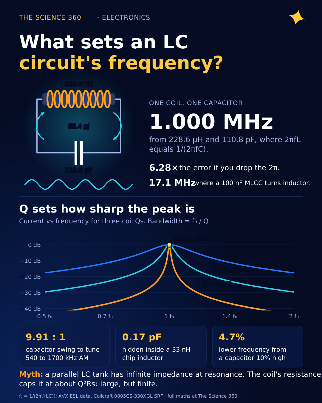
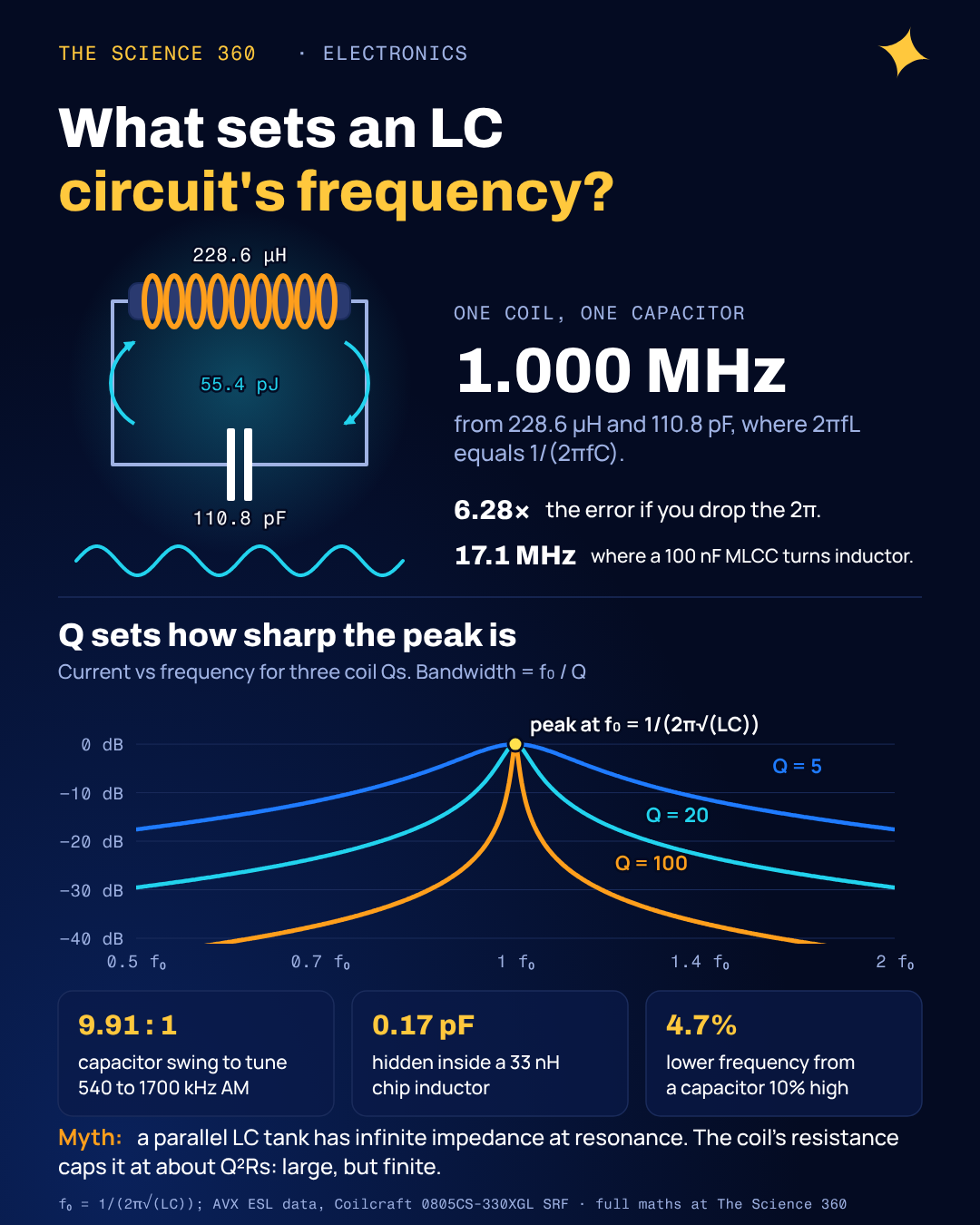
A 228.6 µH coil and a 110.8 pF capacitor, wired together and given one nudge of charge, will swap 55 picojoules back and forth between them a million times a second. That is the whole of LC resonance, and the formula that predicts the million, $f_0 = 1/(2\pi\sqrt{LC})$ , is in every textbook and every online calculator. What the calculators do not tell you is how far a real circuit drifts from it, which version of "resonant frequency" you are actually measuring, and why the capacitor on your bench stops being a capacitor somewhere around 17 MHz.

Quick answerThe resonant frequency of an LC circuit is

f_0 = 1/(2\pi\sqrt{LC})

, with L in henries and C in farads. It is where the inductor's reactance 2πfL equals the capacitor's 1/(2πfC). For example, 228.6 µH with 110.8 pF gives 1.000 MHz. Losses shift a real circuit's zero-phase point slightly below this, by about

1/(2Q^2)

Infographic: What sets an LC circuit's frequency? A coil and a capacitor are wired in a loop, with arrows showing 55.4 pJ of energy swapping between them. 228.6 µH with 110.8 pF resonates at 1.000 MHz, where 2πfL equals 1/(2πfC). Dropping the 2π makes the answer 6.28 times too high. A line chart of resonance curves on a log frequency axis shows the peak at f₀ getting sharper as coil Q rises from 5 to 20 to 100, with bandwidth f₀/Q. Tiles: tuning the AM band needs a 9.91 to 1 capacitor swing, and a capacitor 10% high lowers the frequency 4.7%. — Tap the image to view it full size. View the accessible, editable SVG.

Where does f = 1/(2π√(LC)) come from?

The reactance route is the one most pages use. An inductor's reactance rises with frequency, $X_L = 2\pi f L$ ; a capacitor's falls, $X_C = 1/(2\pi f C)$ . In series they subtract, because one voltage leads the current by 90° and the other lags by 90°. Resonance is where they are equal:

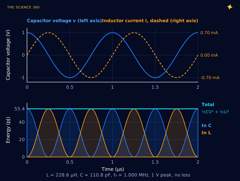
\begin{aligned}2\pi f L &= \frac{1}{2\pi f C} \\ (2\pi f)^2 &= \frac{1}{LC} \\ f_0 &= \frac{1}{2\pi\sqrt{LC}} \\ \omega_0 &= \frac{1}{\sqrt{LC}}\ \ (\mathrm{rad/s})\end{aligned}

The energy route explains why the circuit wants to oscillate at all. Charge a capacitor and connect it across an inductor. Current builds gradually, because the inductor resists any change in current, while the capacitor drains. At zero volts all the energy sits in the magnetic field and the current peaks. The inductor then refuses to let that current stop, so it charges the capacitor the other way round, and the whole thing runs backwards.

Write it as two equations. The inductor says $v = L\,di/dt$ ; the capacitor says $i = -C\,dv/dt$ . Combine them and you get $d^2v/dt^2 = -v/(LC)$ , the equation of a mass on a spring, whose solution is a cosine at $\omega_0 = 1/\sqrt{LC}$ . The inductance plays the role of mass (inertia against changing current) and 1/C plays the role of spring stiffness. Bigger L or bigger C, slower oscillation, and only as the square root.

The energy check is a good way to remember the peak current. At the moment all energy is in the capacitor it is $\tfrac12 C V_0^2$ ; a quarter cycle later it is all $\tfrac12 L I_0^2$ . Set them equal and $I_0 = V_0/\sqrt{L/C}$ . The quantity $\sqrt{L/C}$ has units of ohms and is called the characteristic impedance Z₀ of the resonator. You will meet it again in why coax is 50 Ω, where a transmission line's Z₀ is √(L/C) per unit length.

Worked example: the energy picture at 1 MHz, with L = 228.6 µH, C = 110.8 pF, V₀ = 1 V.

\begin{aligned}\sqrt{LC} &= \sqrt{228.6\,\mu \times 110.8\,\mathrm{p}} \\ &= \sqrt{2.533{\times}10^{-14}} \\ &= 1.5915{\times}10^{-7}\ \mathrm{s} \\ f_0 &= \frac{1}{2\pi \times 1.5915{\times}10^{-7}} \\ &= \mathbf{1.000\ MHz} \\ E &= \tfrac12 \times 110.8\ \mathrm{pF} \times (1\ \mathrm{V})^2 \\ &= \mathbf{55.4\ pJ} \\ Z_0 &= \sqrt{228.6\,\mu\mathrm{H}/110.8\,\mathrm{pF}} \\ &= \sqrt{2.063{\times}10^6} = 1436\ \Omega \\ I_0 &= 1\ \mathrm{V}/1436\ \Omega = \mathbf{0.70\ mA}\end{aligned}

Two stacked plots over 2 microseconds for an ideal 1 megahertz LC circuit. Top: capacitor voltage as a cosine between plus and minus 1 volt and inductor current as a dashed sine between plus and minus 0.70 milliamps, a quarter cycle apart. Bottom: capacitor energy and inductor energy as shaded humps that alternate, each peaking at 55.4 picojoules, with a flat green line showing their constant sum. — Figure 2. Energy sloshing in a lossless 1 MHz LC circuit, computed from $v = V_0\cos(\omega_0 t)$ and $i = (V_0/Z_0)\sin(\omega_0 t)$ . The energy changes hands twice per cycle, so the energy curves run at 2 MHz while the voltage runs at 1 MHz.

The 2π mistake that costs a factor of 6.28

The single most common error with this formula is mixing up f and ω. $1/\sqrt{LC}$ gives angular frequency in radians per second. For the example above, $1/\sqrt{LC} = 6.283 \times 10^6$ , and if you read that as hertz you will build a filter tuned to 6.28 MHz instead of 1 MHz. Simulators report hertz, textbooks often derive in ω, and spreadsheet formulas copied from one into the other are where the factor sneaks in. If your answer is off by 6.28, this is why.

The second common slip is units. Picofarads and microhenries are the natural units for radio work, and their product carries a 10⁻¹⁸. A handy shortcut for exactly those units: $f_0\,[\mathrm{MHz}] = 159.15/\sqrt{L_{\mu\mathrm{H}}\,C_{\mathrm{pF}}}$ . Check: $159.15/\sqrt{228.6 \times 110.8} = 1.000\ \mathrm{MHz}$ .

Series vs parallel LC: what is different?

Two schematics. Left: a series circuit of an AC voltage source, a resistor R, an inductor L and a capacitor C in one loop, labelled Z equals R plus j times omega L minus 1 over omega C, which equals R at resonance. Right: a parallel tank, with a current source feeding a capacitor C in parallel with an inductor L that has a series resistance Rs, labelled Z at resonance equals L over Rs C, equal to Q squared Rs, large but finite. — Figure 1. The two basic resonators. In the series circuit the reactances cancel and only R is left, so the impedance is a minimum. In the parallel tank the branch currents cancel, so the impedance is a maximum. The tank's resistor is drawn in series with the coil because that is where the loss physically lives: the winding resistance.

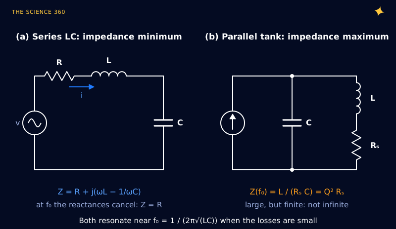
The series circuit is an impedance minimum. At f₀ the inductor's and capacitor's voltages are equal and opposite, so they cancel, and the source sees only R. The parallel circuit is the dual: at f₀ the currents in the two branches are equal and opposite, so the source has to supply only the small current that makes up for losses, and the tank looks like a large resistance.

Both hide a large circulating current or voltage. In a series circuit at resonance the voltage across C is Q times the source voltage, so a Q = 100 circuit driven with 1 V puts 100 V on the capacitor. That is how a wireless charging coil builds a strong magnetic field from a modest supply, and it is also how people blow up 50 V capacitors in circuits fed from 5 V.

The misconception: “at resonance a parallel LC has infinite impedance, and all resonant frequencies are the same”

Most top-ranking pages state the formula, show X_L = X_C, and stop; forum answers often add that a parallel tank has infinite impedance at resonance. Both hold only for perfect parts. Give the coil resistance and two things change.

First, the impedance is finite. For a coil with series resistance R_s, the tank impedance at resonance is very close to $L/(R_s C)$ , which is the same as $Q^2 R_s$ , where $Q = \omega_0 L/R_s$ is the coil's quality factor. Electronics Tutorials gets this right in its parallel resonance page; many shorter answers do not.

Tank impedance at 1 MHz (our numbers, assuming a coil Q of 100):

\begin{aligned}X_L &= 2\pi \times 1\ \mathrm{MHz} \times 228.6\ \mu\mathrm{H} \\ &= 1436\ \Omega \\ R_s &= X_L/Q = 1436/100 = 14.36\ \Omega \\ Z(f_0) &= \frac{L}{R_s C} \\ &= \frac{228.6\ \mu\mathrm{H}}{14.36\ \Omega \times 110.8\ \mathrm{pF}} \\ &= \mathbf{143.7\ k\Omega} \\ Q^2 R_s &= 10\,000 \times 14.36 = 143.6\ \mathrm{k\Omega}\end{aligned}

The last line is a check.

Second, "resonant frequency" stops being one number. With a lossy coil in the tank, there are three reasonable definitions, and they no longer coincide:

The undamped frequency, $\omega_0 = 1/\sqrt{LC}$ , which is the formula.
The zero-phase frequency, where the tank looks purely resistive and the source current is in phase with the voltage: ω = ω₀√(1 − 1/Q²).
The frequency of maximum impedance, which stays within a hair of ω₀ (the exact expression is ω₀√(−1/Q² + √(1 + 2/Q²))).

A fourth number appears if you ring the tank and watch it decay on a scope: the damped natural frequency, $\omega_0\sqrt{1 - 1/(4Q^2)}$ . Here they are for a deliberately poor coil and a good one:

Coil Q = 5, relative to $f_0 = 1/(2\pi\sqrt{LC})$ :

\begin{aligned}\text{zero phase} &= \sqrt{1 - 1/25} \\ &= \mathbf{0.9798\,f_0} \\ \text{max }|Z| &= \sqrt{-0.04 + \sqrt{1.08}} \\ &= \mathbf{0.9996\,f_0} \\ \text{ringing} &= \sqrt{1 - 1/100} \\ &= \mathbf{0.9950\,f_0}\end{aligned}

Those are 2.0%, 0.04% and 0.5% low. At coil Q = 100, zero phase is at 0.99995 f₀ (0.005% low) and ringing at 0.999988 f₀.

We checked the Q = 5 numbers by brute force, sweeping the impedance of $(R_s + j\omega L)$ in parallel with $1/(j\omega C)$ on a fine grid: the peak lands at 0.99962 and the phase crosses zero at 0.97980. So the practical rule is simple. Above a Q of about 20 every definition agrees with $1/(2\pi\sqrt{LC})$ to better than 0.13%, far inside component tolerance, and you can forget the distinction. Below about 10, which is common for ferrite-cored power inductors, lossy wireless charging coils and heavily loaded tanks, it matters: an oscillator that locks to zero phase will run measurably below the formula.

Q and bandwidth: how sharp is the resonance?

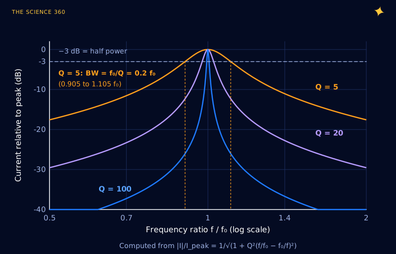
Q measures how many cycles the circuit rings before the energy leaks away. More usefully for design, it sets the bandwidth. The half-power bandwidth, measured between the two frequencies where the response is 3 dB down, is:

\begin{aligned}\text{BW}_{-3\,\mathrm{dB}} &= f_0/Q \\ Q_{\text{series}} &= \frac{1}{R}\sqrt{\frac{L}{C}} = \frac{\omega_0 L}{R} \\ \text{BW} &= \frac{f_0 R}{\omega_0 L} = \mathbf{\frac{R}{2\pi L}}\end{aligned}

The bandwidth is independent of C.

That last line is worth staring at. For a series circuit with a fixed resistance, the bandwidth in hertz depends only on R and L. Retuning with the capacitor moves the centre frequency but leaves the width alone, so Q rises in proportion to frequency. The 3 dB points are not symmetric around f₀ on a linear axis; they are symmetric on a log axis, with their geometric mean equal to f₀. Figure 3 shows the shape for three values of Q. The same half-power definition sets the cutoff of a first-order filter, which is covered in the RC low-pass filter cutoff frequency.

Series RLC current in decibels against frequency ratio from 0.5 to 2 on a log axis for Q of 5, 20 and 100. All three curves peak at 0 dB at f over f0 equal to 1. The Q of 5 curve is broad, crossing minus 3 dB at 0.905 and 1.105; the Q of 100 curve is a narrow spike that falls below minus 40 dB by 0.6 and 1.6. — Figure 3. Resonance curves computed from $|I|/I_{\mathrm{peak}} = 1/\sqrt{1 + Q^2(f/f_0 - f_0/f)^2}$ . Bandwidth at −3 dB is f₀/Q. Far from resonance every curve falls at 20 dB per decade, set by whichever reactance dominates.

Worked example: designing an AM radio tuner

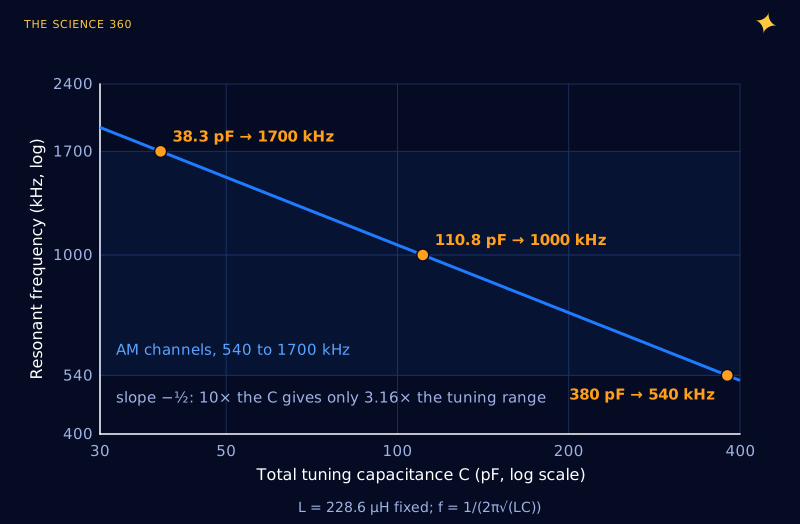
The North American AM broadcast band runs from 535 to 1705 kHz, and its 117 carrier frequencies sit on a 10 kHz grid from 540 to 1700 kHz (FCC rule 47 CFR 73.14). A single variable capacitor and a fixed coil have to cover that range. Because f depends on $1/\sqrt{C}$ , the capacitance range has to be the square of the frequency range:

\begin{aligned}f_{\max}/f_{\min} &= 1700/540 = 3.148 \\ C_{\max}/C_{\min} &= 3.148^2 = \mathbf{9.91 : 1}\end{aligned}

Pick the maximum total capacitance: C_max = 380 pF (our choice, tuning capacitor plus strays).

\begin{aligned}L &= \frac{1}{(2\pi \times 540\ \mathrm{kHz})^2 \times 380\ \mathrm{pF}} \\ &= \frac{1}{1.151{\times}10^{13} \times 3.80{\times}10^{-10}} \\ &= \mathbf{228.6\ \mu H} \\ C_{\min} &= \frac{1}{(2\pi \times 1700\ \mathrm{kHz})^2 \times 228.6\ \mu\mathrm{H}} \\ &= \mathbf{38.3\ pF}\end{aligned}

Mid-band check: 1000 kHz needs 110.8 pF.

The awkward number is C_min. The 38.3 pF is the total: the variable capacitor at its minimum setting plus every stray picofarad from the wiring, the coil's own capacitance and the next stage's input. If strays add 20 pF, the variable capacitor must swing from 18.3 to 360 pF, a ratio near 20:1, which is much harder to make than 10:1. This is why stray capacitance, a nuisance at most frequencies, is a design input for a tuner, and why the same thinking appears in choosing crystal load capacitors, where a few picofarads of board stray decide whether a crystal runs on frequency.

Log-log plot of resonant frequency in kilohertz against total tuning capacitance from 30 to 400 picofarads for a fixed 228.6 microhenry coil. A straight line of slope minus one half passes through 38.3 picofarads at 1700 kilohertz, 110.8 picofarads at 1000 kilohertz and 380 picofarads at 540 kilohertz. The AM band from 540 to 1700 kilohertz is shaded. — Figure 4. On log axes the LC formula is a straight line of slope −½. Ten times the capacitance buys only $\sqrt{10} = 3.16$ times the frequency range, so a 3.15:1 band needs a 9.9:1 capacitor.

Now the selectivity. Suppose the coil's loss behaves like a fixed series resistance chosen to give Q = 100 at 1 MHz, which is R = 14.36 Ω. Then:

\begin{aligned}\text{BW} &= \frac{R}{2\pi L} = \frac{14.36}{2\pi \times 228.6\ \mu\mathrm{H}} \\ &= \mathbf{10.0\ kHz} \\ Q_{540} &= \frac{2\pi \times 540\,\mathrm{k} \times 228.6\,\mu}{14.36} \\ &= 775.6/14.36 = 54 \\ Q_{1700} &= 2441.8/14.36 = 170\end{aligned}

The bandwidth is the same at every setting.

A 10 kHz bandwidth on a 10 kHz channel grid sounds tidy, but a single tuned circuit is a poor channel filter. Look at Figure 3: one channel away (10 kHz off at 1 MHz, which is f/f₀ = 1.01), a Q = 100 circuit is only about 7 dB down: $1/\sqrt{1 + 100^2 (1.01 - 1/1.01)^2} = 0.45$ . A strong local station next door comes straight through. Real coils also do not behave like a fixed resistor; their losses rise with frequency (partly the skin effect in the winding), so the bandwidth varies across the band. This is the reason almost every AM receiver is a superheterodyne: the antenna tank only does rough preselection, and the channel is picked by fixed-frequency filters that do not have to tune.

Source note The coil Q of 100 and the fixed 14.36 Ω loss are our modelling assumptions, chosen to make the arithmetic clean. We did not measure or source the Q of a real ferrite-rod AM antenna; published hobbyist figures vary widely and depend on the rod, the wire and the loading by the next stage.

Why real inductors and capacitors self-resonate

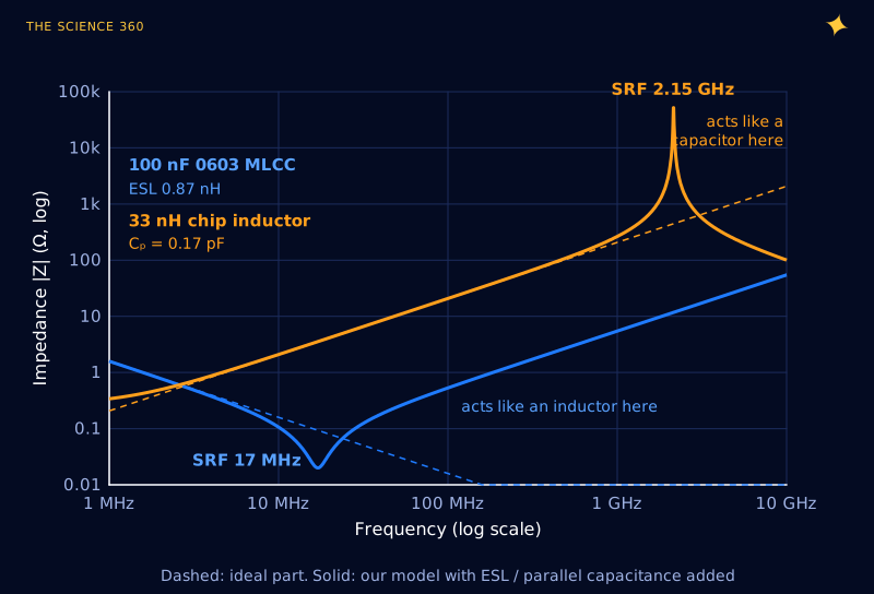
Every real capacitor has some inductance, from the current loop through its plates and terminals. Every real inductor has some capacitance, between adjacent turns. So each part is secretly an LC circuit, with a self-resonant frequency (SRF) of its own. Above that frequency the part does the opposite of its job.

Jeffrey Cain at AVX measured the parasitic inductance of 0.1 µF ceramic capacitors and found about 870 pH for an 0603 chip, 1,050 pH for 0805 and 1,200 pH for 1206. Feed the 0603 number into the formula:

100 nF 0603 MLCC, ESL = 0.87 nH:

\begin{aligned}f_{\mathrm{SRF}} &= \frac{1}{2\pi\sqrt{0.87{\times}10^{-9} \times 100{\times}10^{-9}}} \\ &= \frac{1}{2\pi \times 9.33{\times}10^{-9}} = \mathbf{17.1\ MHz}\end{aligned}

Above 17 MHz that "capacitor" is an inductor of about 0.87 nH plus whatever the board adds, which is exactly the story told in why 100 nF is the standard decoupling capacitor. Going the other way, Coilcraft's 0805CS-330XGL, a 33 nH ceramic chip inductor, is listed with an SRF of 2.15 GHz. Invert the formula to find its hidden capacitance:

\begin{aligned}C_{\mathrm{par}} &= \frac{1}{(2\pi \times 2.15\ \mathrm{GHz})^2 \times 33\ \mathrm{nH}} \\ &= \frac{1}{1.825{\times}10^{20} \times 3.3{\times}10^{-8}} \\ &= \mathbf{0.17\ pF}\end{aligned}

A sixth of a picofarad. That is the whole gap between a 33 nH inductor and an open circuit at 2.15 GHz, and it is why an RF designer picks an inductor whose SRF sits well above the operating frequency, often by a factor of two or more, since the effective inductance climbs steeply as you approach SRF.

Impedance magnitude from 1 megahertz to 10 gigahertz, log scales. A blue curve for a 100 nanofarad 0603 capacitor falls along the ideal dashed capacitor line, reaches a sharp minimum at 17 megahertz, then rises as an inductor. An orange curve for a 33 nanohenry chip inductor rises along the ideal dashed inductor line to a sharp peak at 2.15 gigahertz and then falls like a capacitor. — Figure 5. Both parts are LC circuits in disguise. Capacitor: 100 nF in series with Cain's 0.87 nH ESL and an assumed 20 mΩ ESR. Inductor: 33 nH with the 0.17 pF parallel capacitance implied by its 2.15 GHz SRF and a loss resistance we scaled to give Q ≈ 60 at 500 MHz, near the datasheet's minimum Q. The ESR and loss model are ours.

How accurate does the formula need to be?

Because f₀ goes as the inverse square root, tolerances are halved: a capacitor 10% high moves f₀ 4.7% low ( $\sqrt{1/1.1} = 0.953$ ). That is fine for a filter, but not for a radio that must land within 1% on a 10 kHz grid at 1 MHz, which is why tuners have trimmers and why fixed-frequency oscillators use a quartz crystal, a mechanical resonator with a far higher Q than any coil (see why watch crystals run at 32,768 Hz).

For a stable resonator, use C0G ceramic capacitors and air or low-permeability cores; X7R ceramics and ferrites drift with temperature and bias. Resonance is also how an antenna works, since a quarter-wave whip is a resonant structure with distributed L and C (see quarter-wave antenna length).

The short version for your bench:

f_0 = 1/(2\pi\sqrt{LC})

, or

159.15/\sqrt{L_{\mu\mathrm{H}} C_{\mathrm{pF}}}

in MHz. Watch the 2π. Count stray capacitance in small-C designs. Bandwidth is

f_0/Q

, and for a series circuit

R/(2\pi L)

. A real parallel tank peaks at about Q²R_s, not infinity. Below Q of about 10, expect the zero-phase frequency to sit 1/(2Q²) below the formula. And keep every part's self-resonance well above the frequency you care about.

FAQ

What is the formula for the resonant frequency of an LC circuit?

$f_0 = 1/(2\pi\sqrt{LC})$ , with L in henries, C in farads and f₀ in hertz. The angular frequency is $\omega_0 = 1/\sqrt{LC}$ in radians per second. For example, 228.6 µH with 110.8 pF resonates at 1.000 MHz.

Is the resonant frequency the same for series and parallel LC circuits?

For ideal, lossless parts, yes: both resonate at $1/(2\pi\sqrt{LC})$ . With a lossy coil in a parallel tank the definitions split. The zero-phase frequency drops by a factor $\sqrt{1 - 1/Q^2}$ , about 2% at Q = 5, while the impedance peak stays almost exactly at $1/(2\pi\sqrt{LC})$ . Above Q of about 20 the differences are under 0.13% and can be ignored.

Is the impedance of a parallel LC circuit infinite at resonance?

Only for perfect parts. A real tank has an impedance at resonance of about $L/(R_s C)$ , which equals Q² times the coil's series resistance. A 228.6 µH coil with 14.4 Ω of loss and 110.8 pF gives about 144 kΩ at 1 MHz: large, but finite.

How does Q relate to bandwidth in an LC circuit?

The half-power (−3 dB) bandwidth is f₀/Q. For a series RLC circuit $Q = (1/R)\sqrt{L/C}$ , so the bandwidth works out to $R/(2\pi L)$ , which does not depend on C at all. A Q of 100 at 1 MHz gives a 10 kHz bandwidth.

Why does my LC circuit not resonate at the calculated frequency?

Usually stray capacitance and lead inductance. A few picofarads of wiring and input capacitance can be a large fraction of a small tuning capacitor, and every inductor has its own parallel capacitance that makes it self-resonate. Tolerances of 5 to 20% on L and C shift f₀ by roughly half that percentage, because f₀ depends on the square root.

Sources

Wikipedia, "RLC circuit" (series and parallel Q, bandwidth Δω = R/L, damped frequency ω_d = √(ω₀² − α²), parallel circuit with series coil resistance: zero-phase and maximum-impedance frequencies): en.wikipedia.org/wiki/RLC_circuit
Electronics Tutorials, "Parallel Resonance Circuit" (impedance at resonance is a maximum equal to the circuit resistance, not infinite; coil resistance modifies the formula): electronics-tutorials.ws/accircuits/parallel-resonance.html
Keysight, "Resonance frequency formula" (typical page-one treatment: X_L = X_C, same formula for series and parallel, no Q): keysight.com resonance frequency formula
US Code of Federal Regulations, 47 CFR 73.14 (AM band 535 to 1705 kHz; 117 carriers from 540 to 1700 kHz in 10 kHz steps): law.cornell.edu/cfr/text/47/73.14
Jeffrey Cain, KYOCERA AVX, "Parasitic Inductance of Multilayer Ceramic Capacitors" (0.1 µF ESL: 870 pH 0603, 1,050 pH 0805, 1,200 pH 1206): kyocera-avx.com parasitc.pdf
Coilcraft 0805CS-330XGLC, 33 nH ±2%, Q 60 at 500 MHz, SRF 2.15 GHz, DCR 270 mΩ (distributor listing of the manufacturer data): lcsc.com/product-detail/C38516310.html

Method note: all figures were computed with Python from the equations shown. The AM tuner values (380 pF maximum, coil Q of 100) and the loss models in Figure 5 are our own illustrative choices, not measurements.

Header image: NASA/JPL-Caltech (image PIA17792), regraded for this article.