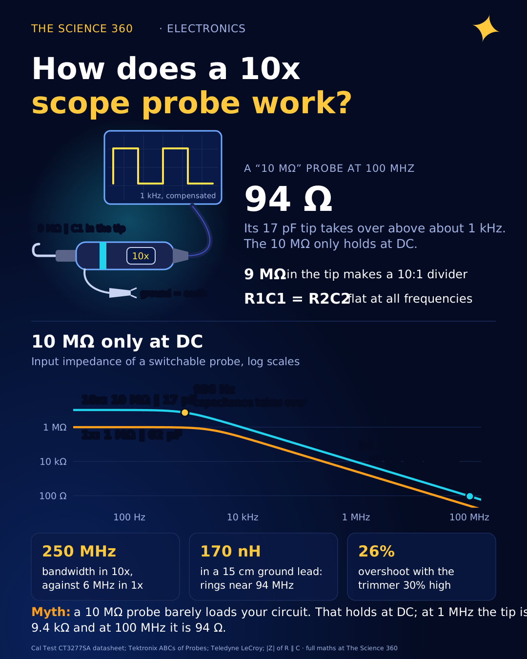
How a 10x Oscilloscope Probe Works (and When It Lies) • The Science 360

Q: How does a 10x oscilloscope probe work?

The probe tip contains a 9 megohm resistor that forms a 10:1 divider with the scope's 1 megohm input. A small adjustable capacitor across the 9 megohm resistor forms a matching capacitive divider with the cable and scope input capacitance, so the division stays 10:1 at all frequencies when R1C1 equals R2C2.

Every new oscilloscope owner is told the same thing on day one: switch the probe to 10x, clip it to the little square-wave tab on the front panel, and twiddle a screw until the waveform looks square. Most people do it once and never think about it again. That screw is the whole design of the probe. Behind it sits a 9 MΩ resistor, a capacitor of about 10 pF, and a piece of arithmetic that has to hold to within a few percent or every edge you look at afterwards is quietly wrong.

The top pages for this question (from Teledyne LeCroy, Rohde & Schwarz and Tektronix) explain the 9 MΩ divider well. What they mostly skip is the capacitor math that makes it work, the fact that a "10 MΩ" probe is under 100 Ω at 100 MHz, and the numbers behind the two classic traps: ground-lead ringing and the ground clip on a mains circuit. This post works through all of them with real component values.

Quick answerA 10x probe puts 9 MΩ in the tip, which forms a 10:1 divider with the scope's 1 MΩ input. An adjustable capacitor across the 9 MΩ forms a matching divider with the cable and input capacitance. When

R_1 C_1 = R_2 C_2

the ratio is 10:1 at every frequency. That trimming is "compensation".

Infographic: How does a 10x scope probe work? A drawing shows a passive probe with its hook tip, 10x switch and ground clip and a scope showing a flat-topped calibration square wave. A 9 megohm tip resistor forms a 10 to 1 divider with the scope's 1 megohm input, and compensation makes R1C1 equal R2C2. A log-scale chart of input impedance shows a 10 megohm, 17 pF probe falling away above 936 Hz and reaching 94 ohms at 100 MHz, with the 1x setting lower still. Tiles: 250 MHz bandwidth in 10x against 6 MHz in 1x; a 15 cm ground lead adds about 170 nH and rings near 94 MHz; a trimmer 30% high gives 26% overshoot. — Tap the image to view it full size. View the accessible, editable SVG.

The 9 MΩ resistor: a 10:1 divider

An oscilloscope input looks like 1 MΩ to ground, in parallel with some capacitance. A 1x probe is just a shielded wire, so your circuit sees that 1 MΩ, plus the capacitance of a metre of coax. A 10x probe adds a 9 MΩ resistor in the tip, so the tip voltage is divided across 9 MΩ and 1 MΩ:

\begin{aligned}V_{\mathrm{scope}} &= V_{\mathrm{tip}} \times \frac{R_2}{R_1 + R_2} \\ &= V_{\mathrm{tip}} \times \frac{1\ \mathrm{M\Omega}}{9\ \mathrm{M\Omega} + 1\ \mathrm{M\Omega}} \\ &= \mathbf{V_{tip}/10}\end{aligned}

DC resistance seen by the circuit:

\begin{aligned}R &= 9\ \mathrm{M\Omega} + 1\ \mathrm{M\Omega} = \mathbf{10\ M\Omega}\end{aligned}

Teledyne LeCroy's explainer points out that "10x" is really a misnomer: it is a 1/10 attenuator, and the scope multiplies the reading back up, either because you told it to or because a sense pin on the probe connector told it. That attenuation costs 20 dB of signal relative to the scope's own noise, which is the real reason 1x still exists.

Ten times the resistance means ten times less DC loading, because the probe forms a divider with the source's own resistance. Tektronix's "ABCs of Probes" primer recommends 10 MΩ for exactly this reason. Our arithmetic for a node with 100 kΩ of source resistance:

10 MΩ probe reads:

\begin{aligned}\frac{10\ \mathrm{M\Omega}}{10\ \mathrm{M\Omega} + 100\ \mathrm{k\Omega}} &= 99.0\%\ \text{of true}\end{aligned}

1 MΩ (1x) reads:

\begin{aligned}\frac{1\ \mathrm{M\Omega}}{1\ \mathrm{M\Omega} + 100\ \mathrm{k\Omega}} &= \mathbf{90.9\%}\end{aligned}

Midpoint of a 100 kΩ / 100 kΩ voltage divider (50 kΩ source): 0.5% low with 10x, 4.8% low with 1x.

Why the resistor alone does not work

If the probe were only a 9 MΩ resistor, it would be useless above a few kilohertz. The scope's 1 MΩ is shunted by its own input capacitance (Teledyne quotes 15 to 17 pF) plus the coax cable, and Teledyne's article says the total at the scope end "can be as much as 100 pF". The 9 MΩ resistor feeding that capacitance is a low-pass filter:

Source resistance seen by C2:

\begin{aligned}R_1 \parallel R_2 &= \frac{9\ \mathrm{M\Omega} \times 1\ \mathrm{M\Omega}}{10\ \mathrm{M\Omega}} = 0.9\ \mathrm{M\Omega} \\ \tau &= 0.9\ \mathrm{M\Omega} \times 90\ \mathrm{pF} = 81\ \mu\mathrm{s} \\ f_{-3\,\mathrm{dB}} &= \frac{1}{2\pi\tau} = \frac{1}{2\pi \times 81\ \mu\mathrm{s}} \\ &\approx \mathbf{2\ kHz}\end{aligned}

A probe that rolls off at 2 kHz would turn a 1 kHz square wave into a shark fin. The same RC math is in our post on the RC low-pass filter cutoff. The fix is to make the capacitance divide in the same ratio as the resistance.

Compensation: why R1C1 = R2C2

Put a capacitor C1 across the 9 MΩ tip resistor (Figure 1). Now there are two dividers in parallel: a resistive one that controls low frequencies and a capacitive one that controls high frequencies. A capacitive divider divides by the inverse ratio of the capacitances, because the smaller capacitor has the larger impedance:

\begin{aligned}\text{Resistive (low } f\text{)}&:\ \frac{R_2}{R_1 + R_2} \\ \text{Capacitive (high } f\text{)}&:\ \frac{C_1}{C_1 + C_2}\end{aligned}

For both to equal 1/10:

\begin{aligned}\frac{C_1}{C_1 + C_2} &= \frac{1}{10} \;\Rightarrow\; C_2 = 9\,C_1\end{aligned}

Since $R_1 = 9\,R_2$ , this is the same as:

\mathbf{R_1 C_1 = R_2 C_2}

With C2 = 90 pF:

\begin{aligned}C_1 &= 90/9 = \mathbf{10\ pF} \\ \tau &= 9\ \mathrm{M\Omega} \times 10\ \mathrm{pF} \\ &= 1\ \mathrm{M\Omega} \times 90\ \mathrm{pF} = 90\ \mu\mathrm{s}\end{aligned}

Schematic of a 10x passive probe. The tip connects to 9 megohms in parallel with an adjustable 10 picofarad capacitor in the probe head, then through a coaxial cable to the scope input, where 1 megohm is in parallel with about 90 picofarads to chassis ground. The coax shield runs to a ground lead and ground clip at the circuit end, and the chassis is tied to mains earth. — Figure 1. The compensated divider. R1 and C1 sit in the probe head; R2 is the scope input and C2 lumps together the scope's input capacitance, the cable and the compensation trimmer. Many probes put the trimmer at the scope end instead, adjusting C2 rather than C1; the condition is the same. Component values are our representative model.

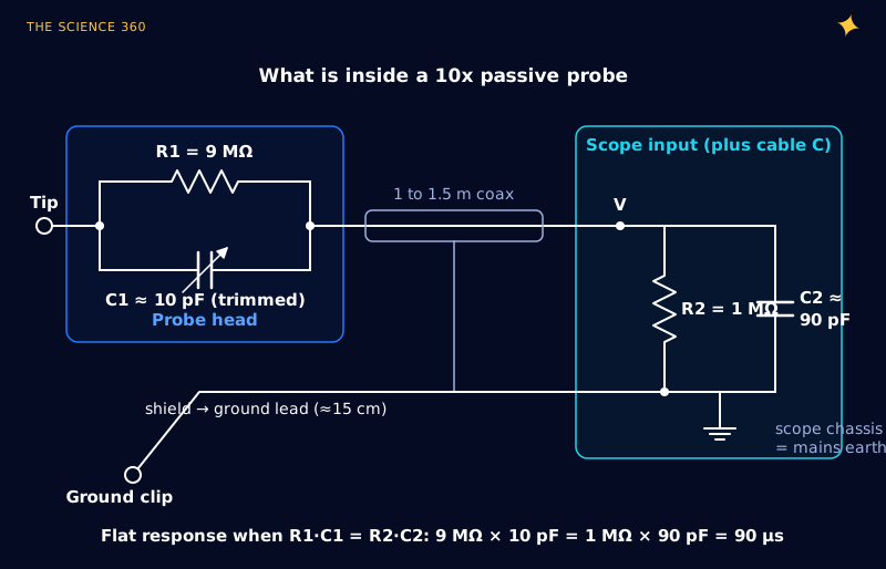
When the two time constants match, the impedances $Z_1 = R_1 \parallel C_1$ and $Z_2 = R_2 \parallel C_2$ are exact scaled copies of each other at every frequency, so their ratio is a constant 1/10. The divider is flat from DC to the point where the cable's transmission-line behaviour and the tip's tiny inductances take over, which is what sets the probe's rated bandwidth.

What the circuit under test sees at high frequency is C1 in series with C2:

\begin{aligned}C_{\mathrm{tip}} &= \frac{C_1 C_2}{C_1 + C_2} = \frac{10 \times 90}{100} \\ &= \mathbf{9\ pF}\end{aligned}

That is how a 10x probe has far less capacitance than a 1x probe on the same cable: the cable capacitance is hidden behind the 10 pF in series. The tip capacitance always comes out as about $C_2/10$ , which matches the 8 to 17 pF figures real 10x probes quote.

Source note The split of C2 between cable, scope input and trimmer varies by probe and by scope, and manufacturers do not publish it. The 90 pF and 10 pF values here are our representative model, chosen to be consistent with Teledyne's "as much as 100 pF" and its 9.5 pF trimmer example. They are not the specification of any particular probe.

What over- and undercompensation look like

The front-panel square wave (usually 1 kHz) is a test of exactly this condition. When a step arrives, the capacitors act first: the output jumps instantly to the capacitive ratio $C_1/(C_1 + C_2)$ . Then the resistors take over, and the output settles exponentially to the resistive ratio of 0.1 with a time constant of $(R_1 \parallel R_2)(C_1 + C_2)$ .

Worked example: a trimmer 30% off. With C2 = 90 pF fixed:

C1 = 7 pF (under):

\begin{aligned}\text{initial step} &= 7/97 = 0.072 \\ \text{final} &= 0.100 \\ &\to \text{edge reaches only } \mathbf{72\%} \\ \tau &= 0.9\ \mathrm{M\Omega} \times 97\ \mathrm{pF} = 87\ \mu\mathrm{s}\end{aligned}

The edge then creeps up with that time constant. C1 = 13 pF (over):

\begin{aligned}\text{initial step} &= 13/103 = 0.126 \\ &\to \mathbf{26\%\ overshoot} \\ \tau &= 0.9\ \mathrm{M\Omega} \times 103\ \mathrm{pF} = 93\ \mu\mathrm{s}\end{aligned}

The overshoot decays with that time constant. At 1 kHz, each half-cycle is $500\ \mu\mathrm{s} \approx 5.5\,\tau$ , long enough to see the whole exponential.

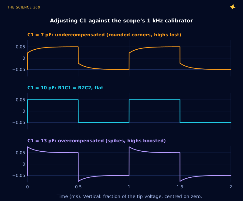
Three simulated scope traces of a 1 kilohertz square wave through a 10x probe. With C1 of 7 picofarads the edges jump only partway and then curve slowly up to the final level, giving rounded corners. With C1 of 10 picofarads the trace is perfectly square. With C1 of 13 picofarads each edge overshoots and then droops back down to the flat level. — Figure 2. Our simulation of the calibrator waveform for three trimmer settings, computed from the step response of the compensated divider. Undercompensation rounds the leading corners; overcompensation adds spikes that droop back. Adjust until the tops are flat.

The Tektronix primer shows the same three shapes and advises compensating whenever you move a probe to a different channel or scope, since each input has slightly different capacitance. The time-domain errors also mean frequency-domain errors: the 30%-under probe reads a 1 MHz sine about 28% low, because at 1 MHz only the capacitive divider matters. If you ever measure ripple or a clock amplitude and the number looks oddly small, check the compensation first.

Why a 10x probe has more bandwidth than 1x

A 1x probe connects the whole cable capacitance directly to your circuit. Cal Test's CT3277SA, a typical switchable 250 MHz probe, lists these figures:

1x: 1 MΩ, 47 pF, bandwidth 6 MHz, rise time 58 ns

10x: 10 MΩ, 17 pF, bandwidth 250 MHz, rise time 1.4 ns

Check (the usual single-pole relation):

\begin{aligned}0.35/58\ \mathrm{ns} &= 6.0\ \mathrm{MHz} \\ 0.35/1.4\ \mathrm{ns} &= 250\ \mathrm{MHz}\end{aligned}

Six megahertz is the probe on its own. Your circuit's source impedance makes it worse, because it charges the probe capacitance. Worked example: probing a node with 1 kΩ of source resistance, adding an assumed 15 pF of scope input to the 1x figure:

1x:

\begin{aligned}\tau &= 1\ \mathrm{k\Omega} \times (47 + 15)\ \mathrm{pF} = 62\ \mathrm{ns} \\ f_{-3\,\mathrm{dB}} &= 1/(2\pi \times 62\ \mathrm{ns}) = \mathbf{2.6\ MHz}\end{aligned}

10x:

\begin{aligned}\tau &= 1\ \mathrm{k\Omega} \times 17\ \mathrm{pF} = 17\ \mathrm{ns} \\ f_{-3\,\mathrm{dB}} &= 1/(2\pi \times 17\ \mathrm{ns}) = \mathbf{9.4\ MHz}\end{aligned}

Rise time $2.2\,\tau$ : 136 ns (1x) versus 37 ns (10x)

Tektronix makes the same point with a 50 Ω, 20 pF pulse source: adding an 11 pF probe raises the measured rise time from 2.2 ns to 3.4 ns, a 55% error. The probe's rated bandwidth is the best case. The circuit's impedance decides what you actually get, and the number that matters for anything fast is the tip capacitance, not the 10 MΩ.

”10 MΩ” only at DC: input impedance versus frequency

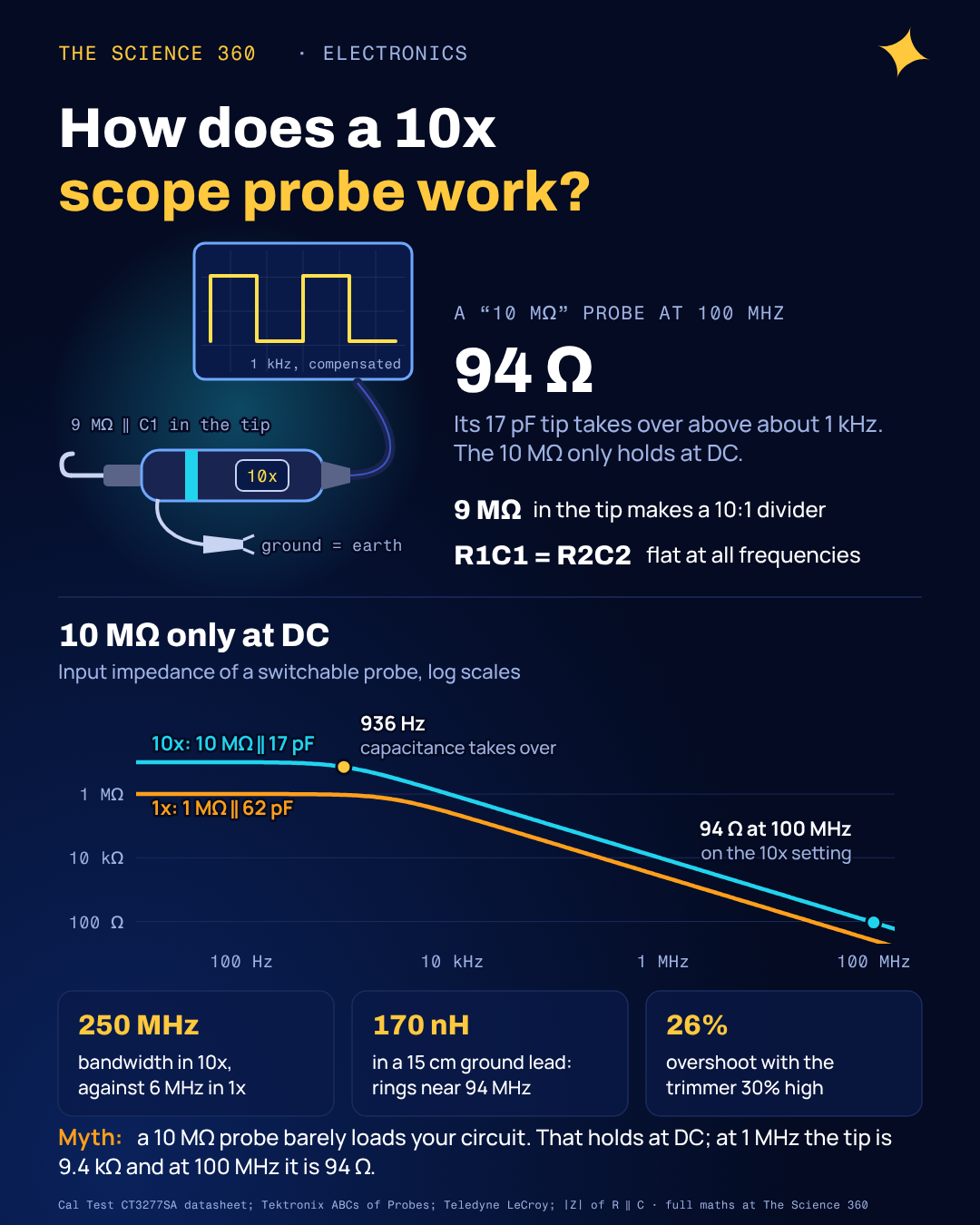
This is the misconception worth correcting. People pick a 10x probe because it is "10 MΩ, so it doesn't load the circuit". At DC that is true. Above about 1 kHz the capacitance takes over, and by radio frequencies the probe is a heavy load:

\begin{aligned}|X_C| &= \frac{1}{2\pi f C},\quad C = 17\ \mathrm{pF}\end{aligned}

Crossover where X_C = 10 MΩ:

\begin{aligned}f &= \frac{1}{2\pi \times 10\ \mathrm{M\Omega} \times 17\ \mathrm{pF}} \\ &= \mathbf{936\ Hz}\end{aligned}

At 1 MHz and at 100 MHz:

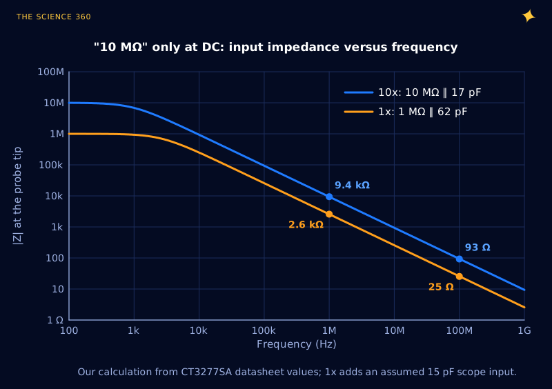
\begin{aligned}|X_C| &= \frac{1}{2\pi \times 10^6 \times 17\ \mathrm{pF}} = \mathbf{9.4\ k\Omega} \\ |X_C| &= \frac{1}{2\pi \times 10^8 \times 17\ \mathrm{pF}} = \mathbf{94\ \Omega}\end{aligned}

Log-log plot of probe input impedance from 100 hertz to 1 gigahertz. The 10x curve starts at 10 megohms, bends down near 1 kilohertz and falls at 20 decibels per decade to 9.4 kilohms at 1 megahertz and 93 ohms at 100 megahertz. The 1x curve starts at 1 megohm and falls to 2.6 kilohms at 1 megahertz and 25 ohms at 100 megahertz. — Figure 3. Input impedance of a $10\ \mathrm{M\Omega} \parallel 17\ \mathrm{pF}$ probe (blue) and a $1\ \mathrm{M\Omega} \parallel 62\ \mathrm{pF}$ probe in 1x mode (orange), our calculation from the CT3277SA figures. By 100 MHz the "10 MΩ" probe presents under 100 Ω.

Ninety-four ohms on a 100 MHz node is not far from terminating a 50 Ω line. On a crystal oscillator it is worse than that: probing the high-impedance side of a crystal adds roughly 17 pF to a circuit whose load capacitance was trimmed in single picofarads (see our crystal load capacitor calculation), so the frequency shifts or the oscillator stops. Tektronix's primer suggests a 10 MΩ probe with 20 pF or less is fine "for most applications", and active FET probes with around 1 pF exist for the rest.

Why the ground lead makes edges ring

The ground lead closes the loop between the probe and your circuit. A 15 cm wire is an inductor, and it forms a series LC circuit with the probe's tip capacitance. Fast edges excite it, and the decaying sine wave you see on top of every edge belongs to the probe, not the circuit. Tektronix describes this ringing as "unavoidable" with a long lead and advises using the shortest ground provided.

Worked example: the standard clip lead. Using the textbook straight-wire inductance formula $L \approx 2\ell\,[\ln(2\ell/r) - 0.75]\ \mathrm{nH}$ , with ℓ and r in centimetres:

15 cm lead, 0.5 mm wire radius:

\begin{aligned}L &\approx 2 \times 15 \times [\ln(600) - 0.75] \\ &= 30 \times 5.65 \approx \mathbf{170\ nH}\end{aligned}

Resonance with 17 pF:

\begin{aligned}f &= \frac{1}{2\pi\sqrt{170\ \mathrm{nH} \times 17\ \mathrm{pF}}} \\ &= \mathbf{94\ MHz}\end{aligned}

Damping from a 50 Ω source:

\begin{aligned}\zeta &= (R/2)\sqrt{C/L} \\ &= 25 \times \sqrt{17\ \mathrm{pF}/170\ \mathrm{nH}} \\ &= 0.25 \to \text{about 44\% overshoot}\end{aligned}

1.5 cm spring ground: L ≈ 10 nH → $f \approx 390\ \mathrm{MHz}$ , $\zeta \approx 1.0$ (no visible ringing)

Ninety-four megahertz is well inside a 250 MHz probe's bandwidth, so the scope shows it faithfully. Figure 4 simulates both cases for a 1 ns edge. The 15 cm lead turns a clean step into a 44% overshoot that rings for 30 ns; the spring tip barely bends. The same LC resonance formula governs both.

Simulated probe voltage versus time from 0 to 40 nanoseconds for a 1 nanosecond step from a 50 ohm source into 17 picofarads. With a 15 centimetre ground lead of about 170 nanohenries the trace overshoots to 1.44, then rings at roughly 94 megahertz for about 30 nanoseconds. With a spring ground of about 10 nanohenries the trace rises cleanly to 1 with no ringing. — Figure 4. Our circuit simulation of a 1 ns edge (dashed) seen through 17 pF of probe capacitance with two ground connections. The ringing on the orange trace is entirely made by the probe.

Source note The 170 nH and 10 nH values are our estimates from the isolated straight-wire formula; the real inductance depends on the loop area formed by the tip, the lead and your circuit's ground path. A Keysight help page reportedly gives a rule of thumb of about 25 nH per inch (about 150 nH for 15 cm), consistent with our estimate, but the page was unavailable when I tried to open it, so I could not confirm the figure.

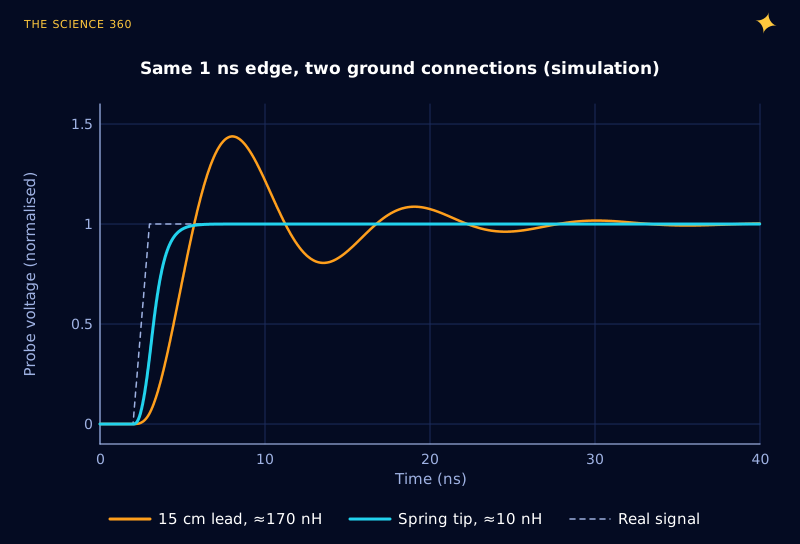
Two practical consequences. If you are measuring switching-regulator ringing (our buck converter post shows where it comes from), the long ground lead can invent ringing or hide the real ringing under its own. Use the spring ground or a ground blade pressed against the nearest ground pad. And the long ground loop also picks up magnetic fields: near a switching inductor it acts as a one-turn coil and adds spikes that vanish when you touch the tip to the ground clip. That test, probing your own ground, is the quickest way to find out how much of what you see is real.

Why you must not clip the ground lead to a mains circuit

On an ordinary bench oscilloscope, the BNC shell is the chassis, and the chassis is bonded to the mains plug's earth pin (Figure 1, bottom right). So the ground clip is not a "negative probe". It is a wire to earth.

In a circuit fed straight from the mains, such as a non-isolated power supply's primary side, a triac dimmer or a motor drive, many nodes sit at hundreds of volts relative to earth. Clip the ground lead to one of them and you have connected that node to earth through the ground lead, the probe's shield and the scope's earth wiring (Figure 5). The only things limiting the current are the wiring resistances, so the result is a fault current of tens or hundreds of amps for the few milliseconds before a fuse, breaker or the ground lead itself gives way.

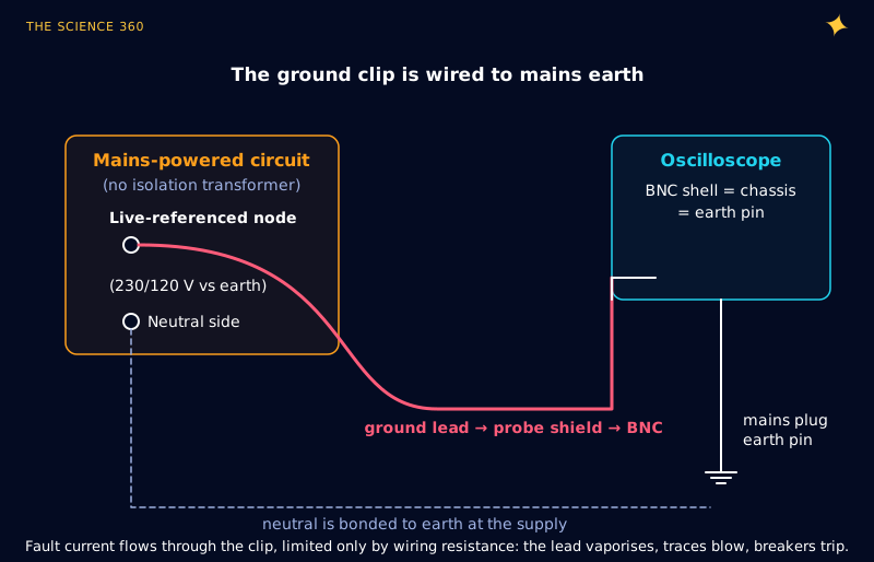
Diagram showing a mains-powered circuit with no isolation transformer and an earthed oscilloscope. A red path runs from a live-referenced node in the circuit, through the probe ground lead and shield, to the scope's BNC shell and chassis and down to the mains plug earth pin. A dashed line shows that the circuit's neutral is bonded to earth at the supply, closing a short-circuit loop. — Figure 5. The ground clip is connected to protective earth through the scope. On any node that is not at earth potential, it completes a short circuit through the probe.

The tempting fix, lifting the scope's earth so the whole instrument floats, is the dangerous one. Tektronix's primer calls it an "unsafe practice" that "allows the oscilloscope chassis to float at potentials that could be a dangerous or deadly shock hazard", and notes the measurements are usually noisy anyway. The safe options are:

A differential probe, which measures between two points without connecting either to earth.
An isolation transformer on the circuit under test (not on the scope), so the circuit no longer has a fixed relationship to earth.
Two channels and the scope's A minus B maths, with both ground clips on earth or left unconnected, for low-frequency work within the probes' voltage ratings.

The same rule explains why birds on a power line are safe: current needs a path between two different potentials. The ground clip supplies exactly that path. Check your probe's voltage rating too: the CT3277SA is rated 300 V CAT II, the category for equipment plugged into ordinary outlets, so it is not for distribution panels or anything upstream.

A checklist for using a 10x probe properly

Use 10x by default. Switch to 1x only for millivolt signals below a few megahertz, where the 20 dB attenuation would put the signal under the scope's noise.
Compensate on each channel you use, with the calibrator square wave, until the tops are flat.
Remember the tip is about 10 to 17 pF. On high-impedance or resonant nodes, that capacitance, not the 10 MΩ, is your loading.
For edges faster than about 10 ns, replace the clip lead with a spring ground and keep the loop small.
Never clip the ground lead to anything that is not at earth potential, and never defeat the scope's earth.

Once the analog front end is right, the scope's sample rate and ADC take over, and those have their own limits, covered in our posts on the Nyquist sampling theorem and on ADC resolution versus accuracy.

The short version: a 10x probe is a

9\ \mathrm{M\Omega} \parallel C_1

divider into the scope's

1\ \mathrm{M\Omega} \parallel C_2

. It is flat when

R_1 C_1 = R_2 C_2

, which is what the compensation screw sets. It loads like 10 MΩ only at DC; at 100 MHz a 17 pF tip is 94 Ω. A 15 cm ground lead adds about 170 nH and rings near 90 to 100 MHz. The ground clip is earth, so keep it off mains-referenced nodes.

FAQ

How does a 10x oscilloscope probe work?

The probe tip contains a 9 MΩ resistor that forms a 10:1 divider with the scope's 1 MΩ input. A small adjustable capacitor across the 9 MΩ resistor forms a matching capacitive divider with the cable and scope input capacitance, so the division stays 10:1 at all frequencies when $R_1 C_1 = R_2 C_2$ .

When should I use 1x instead of 10x?

Use 1x only for small, slow signals, such as a few millivolts of ripple below a few megahertz, where the 20 dB loss of a 10x probe would bury the signal in scope noise. A typical switchable probe has 6 MHz of bandwidth and about 47 pF of loading in 1x, against 250 MHz and 17 pF in 10x.

What happens if a probe is not compensated?

An undercompensated probe rounds the corners of square waves and reads high-frequency signals low. An overcompensated probe adds spikes at each edge and reads high frequencies high. Either way, amplitudes and rise times above a few kilohertz are wrong. Adjust the trimmer on the scope's 1 kHz calibration square wave until the tops are flat.

Why does my oscilloscope show ringing that is not in the circuit?

The ground lead is an inductor, roughly 150 to 200 nH for a 15 cm lead, and it resonates with the probe's tip capacitance. With 17 pF that resonance is near 90 to 100 MHz, inside a 250 MHz probe's bandwidth, so fast edges ring. A short spring ground pushes the resonance far higher.

Can I clip the oscilloscope ground to a mains circuit?

Not to any node that is not at earth potential. On a normal bench scope the ground clip is connected through the BNC shell and chassis to the mains earth pin, so clipping it to a live-referenced node creates a short circuit through the probe. Use a differential probe or an isolation transformer on the circuit, and never disconnect the scope's earth.

Sources

Tektronix, "ABCs of Probes" primer, 60W-6053-17 (resistive loading discussion, probe R and C table, ground-lead ringing and shortest-lead advice, compensation shapes, 2.2 ns to 3.4 ns rise-time example, 10 MΩ with 20 pF or less guidance, floating-scope warning): download.tek.com ABCs of Probes
Teledyne LeCroy, "Secrets of the 10x passive probe explained" (9 MΩ tip resistor, 1 MΩ and 15 to 17 pF scope input, up to 100 pF total, 9.5 pF trimmer example, 1/10 attenuator, 20 dB loss): teledynelecroy.com blog
Rohde & Schwarz, "Understanding passive oscilloscope probes" (10x bandwidth advantage, input capacitance cancellation): rohde-schwarz.com
Cal Test Electronics, CT3277SA 250 MHz switchable probe datasheet (1x/10x: 6/250 MHz, 1/10 MΩ, 47/17 pF, 58/1.4 ns, 300 V CAT II, 15 cm ground lead): CT3277SA datasheet PDF

Method note: Figure 2 is the analytic step response of the compensated divider summed over the square-wave edges. Figure 3 is |Z| of a parallel RC. Figure 4 is a time-step simulation of a 50 Ω source, a series ground-lead inductance and 17 pF. The straight-wire inductance formula $L \approx 2\ell\,[\ln(2\ell/r) - 0.75]\ \mathrm{nH}$ (ℓ, r in cm) is the standard low-frequency approximation for an isolated round wire.

Header image: NASA (image 05pd1613), regraded for this article.