Nyquist Theorem: Why Twice the Frequency Isn't Enough • The Science 360

Q: Why do you need to sample at twice the frequency?

Sampling makes every frequency f indistinguishable from f plus or minus any multiple of the sample rate. Only if all of the signal sits below half the sample rate do those copies avoid landing on top of each other, so the original can be rebuilt uniquely. The real requirement is strictly more than twice the bandwidth, with margin for the anti-alias filter.

Q: What happens if you sample at exactly the Nyquist rate?

A tone at exactly half the sample rate produces samples of A cos(phi) times plus and minus 1. A cosine is captured at full size, a sine aligned with the clock gives all zeros, and anything in between is shrunk. You cannot recover the amplitude and phase, which is why the theorem needs a strict inequality.

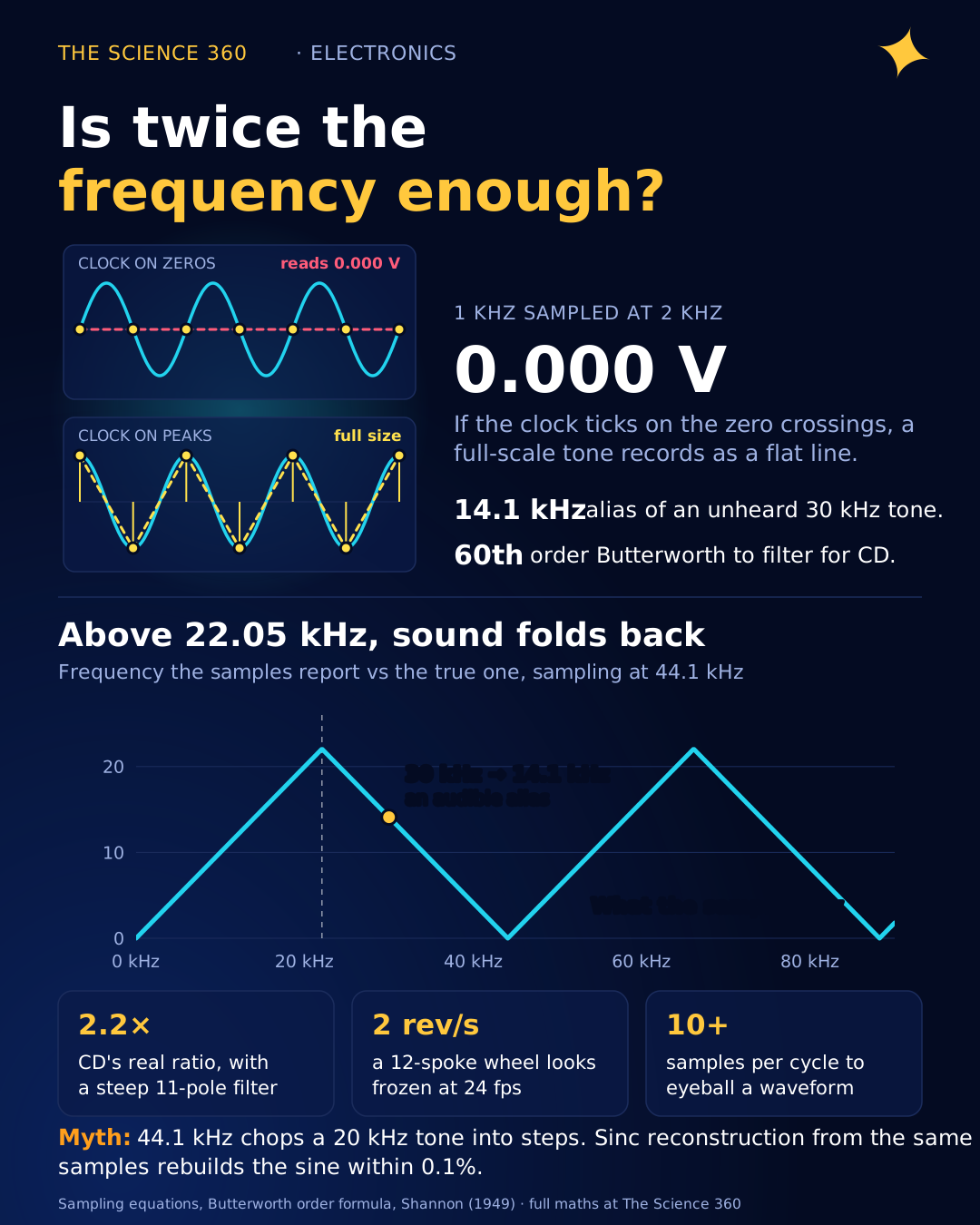
Take a 1 kHz sine wave and sample it at exactly 2 kHz, the rate that "twice the frequency" tells you is enough. If your sample clock happens to tick at the zero crossings, every single sample reads 0.000 V. Your recording of a full-scale tone is a flat line. Shift the clock by a quarter of a cycle and you capture the peaks at full size. Anywhere in between, you get a sine that is too small by an amount you cannot know.

Most pages that rank for this question say "sample at least twice the highest frequency" and stop. The rule is real, but "at least" is wrong, "highest frequency" is a simplification, and the factor of two is a floor that no practical system runs at. Here is where the two comes from, what happens at and above it, and how much faster you actually need to sample.

Quick answerSampling makes a frequency f look identical to

f \pm k f_s

for any whole number k. If the signal has no content at or above

f_s/2

, those copies never overlap and the original can be rebuilt exactly. The condition is strictly more than twice the bandwidth: exactly twice fails, and real systems add margin for the filter.

Infographic: Is twice the frequency enough? Two scope panels show a 1 kHz sine sampled at exactly 2 kHz: with the clock on the zero crossings every sample reads 0.000 V, a flat line, and with the clock on the peaks it is captured at full size. An unheard 30 kHz tone sampled at 44.1 kHz appears as a 14.1 kHz alias, and a Butterworth filter for CD would need order 60. A line chart of reported against true frequency rises to 22.05 kHz, then folds down and zig-zags. Tiles: CD samples at 2.2 times 20 kHz, a 12-spoke wheel looks frozen at 2 rev/s on 24 fps film, and eyeballing a waveform takes 10 or more samples per cycle. — Tap the image to view it full size. View the accessible, editable SVG.

Where does the factor of two come from?

One sample tells you the value of the signal at one instant and nothing about what it did in between. So ask which sinusoids pass through a given set of samples taken every $T_s = 1/f_s$ seconds. Write a cosine at frequency f and evaluate it only at the sample times $t = n T_s$ :

x[n] = \cos(2\pi f n/f_s)

Replace f by $f + k f_s$ :

\begin{aligned}&\cos(2\pi f n/f_s + 2\pi k n) \\ &= \cos(2\pi f n/f_s)\end{aligned}

because $k n$ is a whole number. Replace f by $k f_s - f$ :

\begin{aligned}&\cos(2\pi k n - 2\pi f n/f_s) \\ &= \cos(2\pi f n/f_s)\end{aligned}

because cosine is even. So $f,\ f_s - f,\ f_s + f,\ 2f_s - f, \dots$ all give the same samples.

Every frequency has an infinite family of impostors that produce the same numbers, and the samples cannot say which one was really there. The only way to make the answer unique is to promise, in advance, that the signal lives in a range where each family has exactly one member. The ranges 0 to $f_s/2$ , $f_s/2$ to $f_s$ , $f_s$ to $3f_s/2$ and so on each contain one representative of every family, and the lowest one is the natural choice. Hence the rule: keep everything below $f_s/2$ , the Nyquist frequency, or equivalently sample faster than twice the highest frequency, the Nyquist rate.

In frequency-domain language: sampling repeats the spectrum at every multiple of f_s, a band from −B to +B is 2B wide, and the copies overlap unless $f_s \gt 2B$ .

Why does sampling at exactly twice the frequency fail?

The edge case is where the copies "just touch", and it is worth doing with numbers because it shows why the inequality has to be strict. Let the tone sit exactly at $f_s/2$ , with amplitude A and an unknown phase φ:

x(t) = A\cos(2\pi (f_s/2)\,t + \varphi)

At $t = n/f_s$ :

\begin{aligned}x[n] &= A\cos(\pi n + \varphi) \\ \cos(\pi n + \varphi) &= \cos(\pi n)\cos\varphi \\ &\quad - \sin(\pi n)\sin\varphi \\ &= (-1)^n\cos\varphi\end{aligned}

since $\sin(\pi n) = 0$ . So:

x[n] = (A\cos\varphi)\cdot(-1)^n

The samples alternate +c, −c, +c, −c, and the only thing they record is the product $c = A\cos\varphi$ . A 1 V cosine ( $\varphi = 0$ ) gives ±1.00. A 1.41 V tone at $\varphi = 45^\circ$ gives the same ±1.00. A 10 V sine ( $\varphi = 90^\circ$ ) gives all zeros. Figure 1 shows three of these cases. Two numbers, amplitude and phase, have been squeezed into one, and the information is gone.

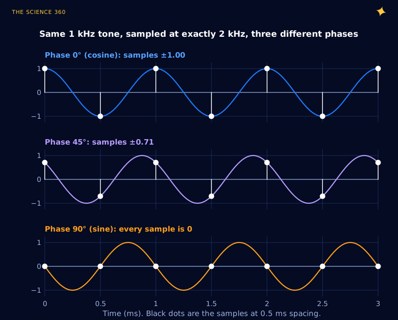
Three stacked plots of a 1 kHz sinusoid sampled at exactly 2 kHz over 3 milliseconds. With phase 0 (cosine) the samples alternate plus and minus 1. With phase 45 degrees they alternate plus and minus 0.71. With phase 90 degrees (sine) every sample lands on a zero crossing and reads 0. — Figure 1. At exactly $f_s = 2f$ , what you capture depends on where the clock happens to land. The samples only report $A\cos\varphi$ , so a sine at the Nyquist frequency can vanish completely.

Shannon's own 1949 statement in the Proceedings of the IRE reads: "If a function f(t) contains no frequencies higher than W cps, it is completely determined by giving its ordinates at a series of points spaced 1/2W seconds apart." Read literally, "no higher than W" allows a component at exactly W, and Figure 1 is the counterexample. Modern statements require $f_s \gt 2B$ strictly: twice is the boundary, not a working point. Shannon also credited the idea in approximate form to Harry Nyquist, whose 1928 paper "Certain topics in telegraph transmission theory" gave the name we now use.

What is aliasing, and where does a frequency end up?

When a tone breaks the rule, it does not disappear. It shows up as a different, lower frequency, the member of its family that lies between 0 and $f_s/2$ . That impostor is called an alias. Figure 2 is the classic demonstration: a 7 kHz tone sampled at 8 kHz.

Alias frequency: $f_a = |f - k f_s|$ , with k the whole number that makes $f_a \le f_s/2$ .

7 kHz sampled at 8 kHz, k = 1:

f_a = |7 - 8| = \mathbf{1\ kHz}

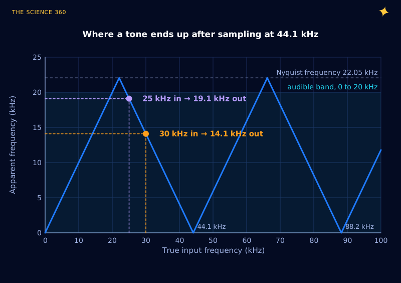
30 kHz sampled at 44.1 kHz, k = 1:

f_a = |30 - 44.1| = \mathbf{14.1\ kHz}

50 kHz sampled at 44.1 kHz, k = 1:

f_a = |50 - 44.1| = \mathbf{5.9\ kHz}

A 7 kHz sine wave over 1 millisecond with black dots at 8 kHz sample instants every 125 microseconds. A dashed orange 1 kHz inverted sine passes exactly through every dot, showing the two signals give identical samples. — Figure 2. Every sample of the 7 kHz input (blue) also lies on a 1 kHz sine (dashed orange). After sampling, nothing distinguishes them, and any reconstruction will produce the 1 kHz version.

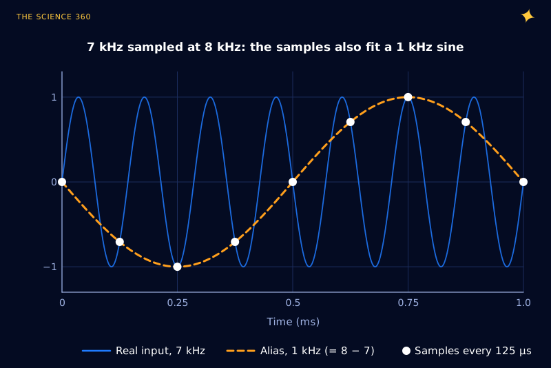
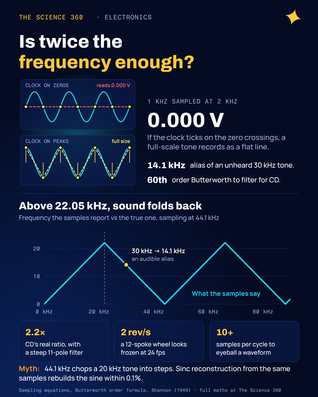
The mapping from true frequency to apparent frequency is a triangle wave, shown in Figure 3 for the CD rate. Frequencies rise normally up to 22.05 kHz, then fold back down, hit zero at 44.1 kHz, rise again and keep zig-zagging. Engineers call this folding, and it is why the Nyquist frequency is sometimes called the folding frequency. Note what the 30 kHz example means in practice: an ultrasonic tone nobody can hear becomes a 14.1 kHz whistle that everyone can.

Triangle-shaped plot of apparent frequency versus true input frequency for sampling at 44.1 kilohertz. The line rises from 0 to 22.05 kilohertz, folds back to 0 at 44.1 kilohertz, rises again to 22.05 at 66.15, and returns to 0 at 88.2. Markers show 25 kilohertz appearing at 19.1 kilohertz and 30 kilohertz at 14.1 kilohertz, both inside the shaded audible band. — Figure 3. Folding at 44.1 kHz, computed from $f_a = |f - k f_s|$ . Anything above 24.1 kHz folds back into the audible band unless a filter removes it first.

Two consequences are easy to miss. First, aliasing cannot be undone after the fact. The 14.1 kHz alias and a genuine 14.1 kHz note give identical numbers, so a digital filter downstream has no handle to grab. The only cure is an analog low-pass filter in front of the ADC, which is why it is called an anti-alias filter (the same RC math as in our post on the RC low-pass filter cutoff, scaled up to many poles). Second, aliasing also hits noise. Broadband noise from DC to 1 MHz, sampled at 44.1 kHz with no filter, folds every slice of that megahertz into the 0 to 22 kHz band, which raises the noise floor even when there are no ultrasonic tones at all.

Why the “wagon wheel” spins backwards

A film camera is a sampler with f_s equal to its frame rate, and a spoked wheel is a periodic signal. The aliasing math explains the old Western stagecoach scene exactly. Take a 12-spoke wheel filmed at 24 frames per second. The pattern repeats every 1/12 of a turn, so the "signal frequency" is 12 times the rotation rate.

Pattern frequency is $12 \times \text{rotation rate}$ (rev/s). The wheel looks frozen when the pattern frequency is 24 Hz:

\text{rotation} = 24/12 = \mathbf{2\ rev/s}

With a 0.65 m tyre:

\begin{aligned}\text{circumference} &= \pi \times 0.65 = 2.04\ \mathrm{m} \\ \text{speed} &= 2 \times 2.04 = 4.1\ \mathrm{m/s} \\ &\approx \mathbf{14.7\ km/h}\end{aligned}

At 1.8 rev/s:

\begin{aligned}\text{pattern} &= 21.6\ \mathrm{Hz} \\ \text{alias} &= 21.6 - 24 = -2.4\ \mathrm{Hz}\end{aligned}

so the spokes creep backwards at $2.4/12 = 0.2$ rev/s.

At 2.2 rev/s:

\begin{aligned}\text{pattern} &= 26.4\ \mathrm{Hz} \\ \text{alias} &= +2.4\ \mathrm{Hz}\end{aligned}

so the spokes creep forwards at 0.2 rev/s.

The negative sign is the thing to notice. An alias carries direction as well as frequency, and for a rotating pattern that shows up as reversed motion. A strobe "freezing" a spinning pulley is the same arithmetic.

How much faster than twice do you really need to sample?

The theorem assumes a brick-wall filter that passes everything below $f_s/2$ and nothing above. That filter cannot be built (its impulse response stretches infinitely into the past), so real filters roll off over a transition band, and the width of that band sets the practical sample rate.

Worked example: the anti-alias filter for CD audio. Suppose you want to keep 0 to 20 kHz and want any aliases landing in that band to sit 96 dB down, about the range of 16-bit audio. Using Figure 3, a frequency only folds into 0 to 20 kHz if it is above $f_s - 20\ \mathrm{kHz}$ . So the filter must be flat-ish at 20 kHz and 96 dB down at 24.1 kHz.

Butterworth magnitude, with $f_c = 20\ \mathrm{kHz}$ (the −3 dB point):

|H|^2 = \frac{1}{1 + (f/f_c)^{2n}}

Need 96 dB at 24.1 kHz:

\begin{aligned}(24.1/20)^{2n} &\ge 10^{9.6} \\ 2n \cdot \log_{10}(1.205) &\ge 9.6 \\ 2n \times 0.0810 &\ge 9.6 \\ n &\ge 59.3\end{aligned}

Butterworth order needed: 60 (a hopeless analog filter)

Elliptic filter, 0.1 dB passband ripple, same corners (our scipy calculation): 11th order

At 48 kHz:

\begin{aligned}\text{ratio} &= 28/20 = 1.4 \\ n &\ge 9.6/(2 \times 0.146)\end{aligned}

which gives Butterworth 33, elliptic 10.

Even the elliptic answer is an eleven-pole analog filter with tight tolerances and ugly phase near 20 kHz. Figure 4 shows how fast the problem eases as the sample rate rises.

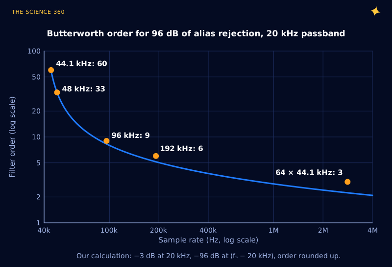
Log-log design chart of required Butterworth filter order versus sample rate from 40 kilohertz to 4 megahertz for a 20 kilohertz passband and 96 decibels of rejection at the first alias band. Marked points: 44.1 kilohertz needs order 60, 48 kilohertz order 33, 96 kilohertz order 9, 192 kilohertz order 6, and 64 times 44.1 kilohertz needs only order 3. — Figure 4. Required Butterworth order versus sample rate, our calculation using $n = \log_{10}(10^{A/10} - 1) / (2\log_{10}((f_s - 20\,\mathrm{kHz})/20\,\mathrm{kHz}))$ with $A = 96\ \mathrm{dB}$ . Oversampling turns an impossible filter into a trivial one.

This is why nearly every modern audio ADC is a delta-sigma converter that samples internally at many megahertz. At $64 \times 44.1\ \mathrm{kHz} = 2.8224\ \mathrm{MHz}$ the first alias band starts around 2.8 MHz, and the ratio becomes $2{,}802/20 = 140$ :

\begin{aligned}n &\ge 9.6/(2 \times \log_{10}140) \\ &= 9.6/(2 \times 2.146) \\ &= 2.24 \;\Rightarrow\; \mathbf{3rd\ order}\end{aligned}

A one-pole RC gets you a good part of the way.

The steep filtering then happens in the digital domain, where an extra hundred filter taps cost silicon area rather than precision capacitors. TI's ADS131M08 datasheet makes exactly this argument for its own delta-sigma ADC: because the integrated digital filter strongly attenuates everything except the region near the modulator frequency, "a single-order RC filter provides sufficient antialiasing protection in the vast majority of applications". A legacy National Semiconductor note now hosted by TI (SNOA350) puts numbers on the contrast: a Nyquist-rate ADC's filter "typically must have a flat response up to about $0.45 \times f_S$ and attenuate all frequencies above $0.5 \times f_S$ " to below the noise floor, while a 64× oversampling converter pushes the critical attenuation point out by a factor of 127. The sample rate you end up storing is still 44.1 or 48 kHz. Oversampling just moves the hard work to where it is cheap. It is also one of the tricks behind the noise numbers in our post on ADC resolution versus accuracy.

Why is CD audio 44.1 kHz and not 40 kHz?

Human hearing is usually quoted as reaching about 20 kHz, so the Nyquist rate is 40 kHz. The extra 4.1 kHz is the filter's transition band: 44.1 kHz leaves a 2.05 kHz gap between 20 kHz and the Nyquist frequency of 22.05 kHz, and, as worked above, frequencies up to 24.1 kHz can be attenuated without their aliases reaching the audio band. Without that margin, Figure 4's curve goes vertical.

The oddly specific value comes from history. Early digital audio masters were stored as black-and-white video on video recorders, through "PCM adaptors". The rate had to fit a whole number of samples into each usable video line:

Usable lines per field × fields per second × samples per line:

\begin{aligned}\text{625-line, 50 Hz}&:\ 294 \times 50 \times 3 \\ &= \mathbf{44{,}100\ samples/s} \\ \text{525-line, 60 Hz}&:\ 245 \times 60 \times 3 \\ &= \mathbf{44{,}100\ samples/s}\end{aligned}

The same number works for both television systems. It also factorises prettily: $44{,}100 = 2^2 \times 3^2 \times 5^2 \times 7^2$ .

Source note The video-adaptor origin and the line counts above come from secondary sources (Watkinson's The Art of Digital Audio as cited by Wikipedia, and Henning Schulzrinne's Columbia notes). I did not find a Sony or Philips primary document stating the reasoning. The claim that early CD players used analog brick-wall filters of roughly 9th to 11th order is also widely repeated; my elliptic calculation is consistent with it, but I did not confirm a specific player's schematic.

The staircase myth: does 44.1 kHz chop a 20 kHz tone into steps?

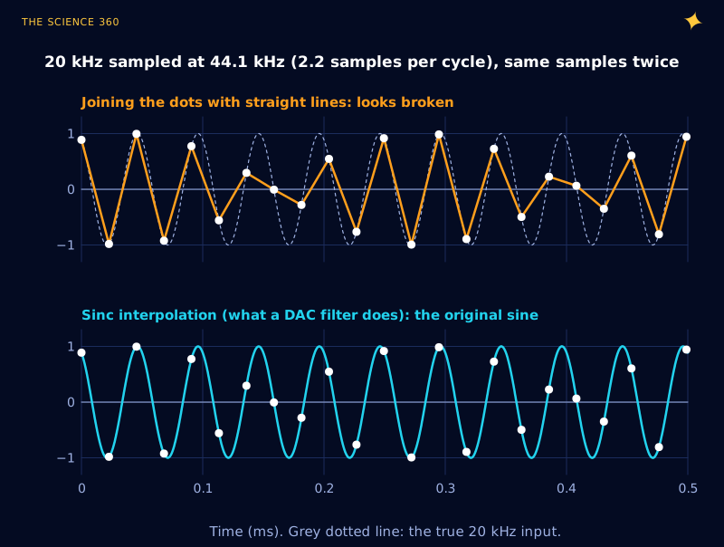
The second misconception sits on the output side. Join the dots of a 20 kHz tone sampled at 44.1 kHz and you get a wobbling, half-broken wave with what looks like a 4.1 kHz beat (Figure 5, top). People see that plot and conclude that high frequencies on a CD are crude approximations.

But joining dots is not what the theorem says to do. The Whittaker-Shannon reconstruction places a sinc pulse, $\sin(\pi x)/(\pi x)$ , at every sample and adds them up. A real DAC approximates this with its reconstruction filter. Do that with the same samples and the original 20 kHz sine comes back (Figure 5, bottom). In our simulation, using 4,000 samples, the reconstructed wave matches the true sine to within 0.1% in the window shown. The information was always there; straight lines just are not the right way to read it.

Two plots of the same samples of a 20 kilohertz sine taken at 44.1 kilohertz. Top: straight orange lines between the samples form an irregular wave with a slow 4.1 kilohertz wobble in amplitude. Bottom: a green sinc-interpolated curve through the same samples is a clean 20 kilohertz sine that matches the dotted true input. — Figure 5. Same 23 samples, two ways of filling the gaps. Linear interpolation (top) gives a false beat. Sinc interpolation (bottom, our numerical reconstruction from 4,000 samples) recovers the input to within 0.1%.

Joining the dots is still how most plotting tools draw sampled data, so it is useful to know how wrong it can be. The worst-case error is at a peak that falls halfway between two samples:

k = samples per cycle; samples either side of the peak sit at $\pm\pi/k$ radians.

\begin{aligned}\text{joined-dot peak} &= \cos(\pi/k) \\ \text{error} &= 1 - \cos(\pi/k)\end{aligned}

\begin{aligned}k = 2.2&:\ 1 - \cos(81.8^\circ) = \mathbf{86\%}\ \text{low} \\ k = 4&:\ 1 - \cos(45^\circ) = 29\%\ \text{low} \\ k = 10&:\ 1 - \cos(18^\circ) = \mathbf{4.9\%}\ \text{low} \\ k = 20&:\ 1 - \cos(9^\circ) = 1.2\%\ \text{low}\end{aligned}

That is the rule of thumb for eyeballing waveforms: if you want the picture to look like the signal without sinc reconstruction, aim for 10 or more samples per cycle. Our post on the 10x oscilloscope probe covers the analog front end that sits before the scope's sampler.

Is it the highest frequency or the bandwidth that matters?

Strictly, it is the bandwidth. The "highest frequency" version is the special case where the band starts at 0 Hz. A signal confined between 100 and 102 MHz, like an FM broadcast channel, occupies only 2 MHz of spectrum. Wikipedia's treatment of non-baseband sampling uses exactly that example: sampling at 4 MHz is enough. The alias formula shows why: with $k = 25$ , 100.5 MHz lands at 0.5 MHz and 101.5 MHz at 1.5 MHz, so the whole channel folds onto 0 to 2 MHz without overlapping itself.

Software-defined radios use this deliberately (bandpass sampling, or undersampling). It only works when the band sits in the right place relative to multiples of $f_s/2$ , and it still needs a bandpass filter to keep the other zones of Figure 3 empty. Aliasing is a deterministic mapping: you either prevent it or exploit it.

A checklist for choosing a sample rate

A working engineer's version of the theorem:

Decide the bandwidth B you actually care about, not the highest frequency that might be present.
Decide how far down aliases must be, usually to the noise floor of the converter (about 6 dB per bit).
Pick f_s so that $f_s - B$ leaves room for a filter you can build. For a simple two- or three-pole filter that typically means 5 to 10 times B, or a delta-sigma ADC that oversamples internally.
Remember that interference counts too. Mains hum at 50 or 60 Hz and its harmonics (see why mains is 50 or 60 Hz) and switching regulator noise at hundreds of kilohertz will alias down to wherever Figure 3 sends them.
If you only need to look at a waveform, plan for 10 or more samples per cycle.

If the anti-alias filter is an active one, the op-amp's bandwidth limits how well it rejects at high frequency, which is where the gain-bandwidth product comes in. Sampled audio loops such as noise-cancelling headphones add a further constraint: every filter adds delay.

The short version: sampling cannot tell f from

f_s \pm f

, so all content must stay strictly below

f_s/2

. At exactly 2× a sine can vanish. Anything above

f_s/2

folds back as an alias that no later processing can remove. The factor you really need depends on your anti-alias filter: 2.2× for CD audio with an aggressive filter, far more if the filter is simple.

FAQ

Why do you need to sample at twice the frequency?

Sampling makes every frequency f indistinguishable from $f \pm k f_s$ . Only if all of the signal sits below half the sample rate do those copies avoid landing on top of each other, so the original can be rebuilt uniquely. The real requirement is strictly more than twice the bandwidth, with margin for the anti-alias filter.

What happens if you sample at exactly the Nyquist rate?

A tone at exactly $f_s/2$ produces samples of $A\cos\varphi \times (-1)^n$ . A cosine is captured at full size, a sine aligned with the clock gives all zeros, and anything in between is shrunk. You cannot recover the amplitude and phase, which is why the theorem needs a strict inequality.

Why is CD audio sampled at 44.1 kHz?

44.1 kHz gives a 2.05 kHz gap above the 20 kHz audio band for the anti-alias filter to work in. The exact number comes from early digital audio stored on video recorders: 3 samples per line on 294 lines at 50 fields per second, or 245 lines at 60 fields per second, both equal 44,100 samples per second.

Can aliasing be removed after sampling?

Not in general. Once a 30 kHz tone has been sampled at 44.1 kHz it produces exactly the same numbers as a real 14.1 kHz tone, so no digital filter can tell them apart. Aliasing has to be prevented with an analog low-pass filter before the ADC.

Why do wheels look like they spin backwards on video?

The camera samples the wheel at its frame rate. A 12-spoke wheel filmed at 24 frames per second looks frozen at exactly 2 revolutions per second, because each spoke moves to the next spoke's position between frames. Slightly slower and each spoke falls just short, so the pattern appears to creep backwards.

Sources

C. E. Shannon, "Communication in the Presence of Noise", Proc. IRE 37(1), 1949, reprinted Proc. IEEE 86(2), 1998 (Theorem 1 wording, credit to Nyquist and Gabor): reprint PDF (University of Miami)
Wikipedia, "Nyquist-Shannon sampling theorem" (strict inequality, the $\cos(2\pi Bt + \theta)$ critical-frequency family, 100 to 102 MHz bandpass example): en.wikipedia.org/wiki/Nyquist-Shannon_sampling_theorem
Wikipedia, "44,100 Hz" (2.05 kHz transition band, PAL 294 × 50 × 3 and NTSC 245 × 60 × 3, citing Watkinson, The Art of Digital Audio, 1989): en.wikipedia.org/wiki/44,100_Hz
Henning Schulzrinne, Columbia University, "Explanation of 44.1 kHz CD sampling rate" (video line arithmetic, filter margin, 2²3²5²7²): cs.columbia.edu/~hgs/audio/44.1.html
Texas Instruments, ADS131M08 datasheet, antialiasing section ("a single-order RC filter provides sufficient antialiasing protection"): ti.com ADS131M08 datasheet
Texas Instruments (National Semiconductor legacy), SNOA350, on oversampling converters and relaxed anti-alias requirements: ti.com/lit/pdf/snoa350

Method note: Figures 1 to 3 and 5 are computed directly from the sampling equations with numpy. Figure 5's reconstruction sums unwindowed sinc pulses over 4,000 samples. Filter orders in Figure 4 and the text are our calculations from the Butterworth formula; elliptic orders are from scipy.signal.ellipord with 0.1 dB passband ripple and 96 dB stopband.

Header image: NASA/JPL-Caltech/ASU/MSSS (image PIA25881), regraded for this article.