Op Amp Gain Bandwidth Product Explained (Noise Gain) • The Science 360

Q: Why does an inverting amplifier with gain -1 have half the bandwidth?

Bandwidth depends on the noise gain, 1 + Rf/Rin, which is the gain the op amp applies to a signal at its non-inverting input. A gain of -1 uses equal resistors, so its noise gain is 2 and its bandwidth is half the gain bandwidth product, while a +1 buffer has noise gain 1 and the full bandwidth.

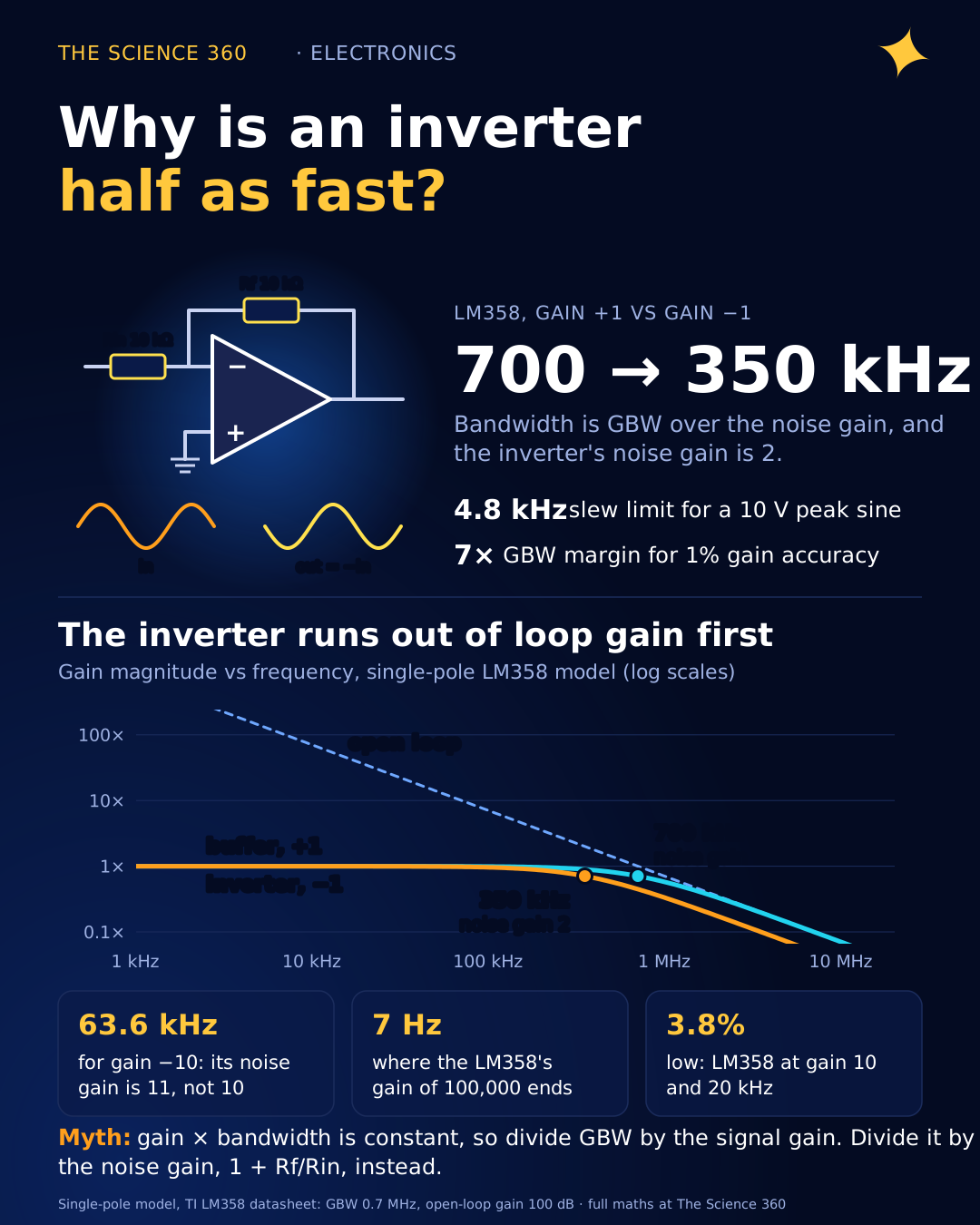
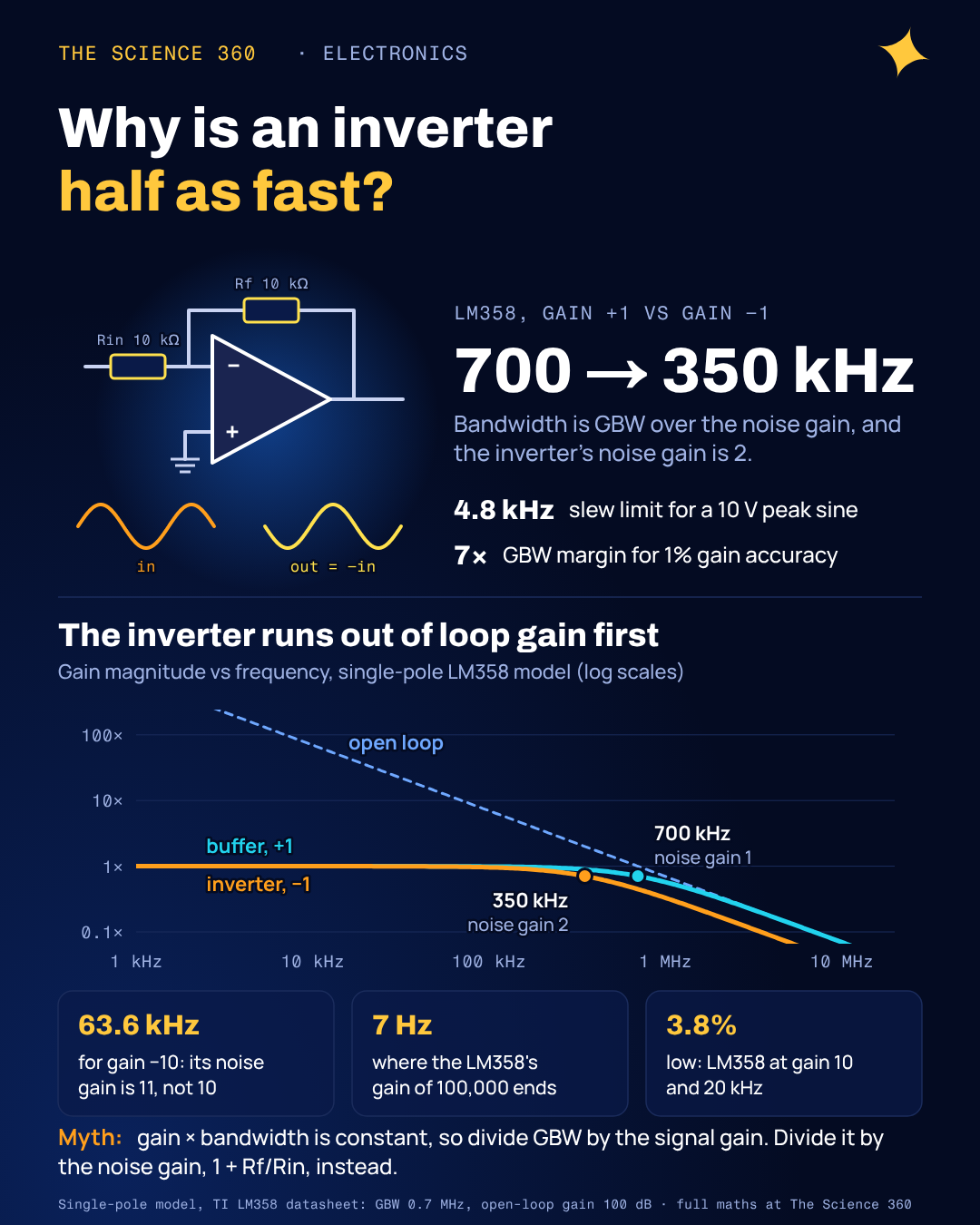
Build an inverting amplifier with two 10 kΩ resistors around an LM358, a gain of −1, and measure its bandwidth. You will get about 350 kHz. Now rewire the same op amp as a plain unity-gain buffer, gain +1, and you get about 700 kHz. Same chip, same gain magnitude, twice the bandwidth. If gain bandwidth product means "gain times bandwidth is constant", one of those measurements has to be wrong.

Neither is. The rule works, but it is easy to multiply by the wrong gain. The top results for this question are mostly distributor glossary entries and short videos that stop at " $\text{gain} \times \text{bandwidth} = \text{constant}$ ". This post does the version that survives contact with a real circuit: which gain to use, how much bandwidth you actually need for accurate gain, where the rule bends at low gain, and why slew rate can wreck a signal long before the bandwidth limit.

Quick answerGain bandwidth product (GBW) is the frequency at which a single-pole op amp's open-loop gain falls to 1. With feedback, the closed-loop bandwidth is roughly GBW divided by the noise gain,

1 + R_f/R_{in}

, not by the signal gain. So a gain of −1 gets

\mathrm{GBW}/2

. For large signals, check slew rate separately: a sine needs

2\pi f V_{\mathrm{peak}}

Infographic: Why is an inverter half as fast? An op-amp triangle is wired as an inverting amplifier with two 10 kΩ resistors, turning an input sine upside down. The same LM358 has 700 kHz of bandwidth as a gain +1 buffer but 350 kHz as a gain −1 inverter, because bandwidth is the 0.7 MHz gain bandwidth product divided by the noise gain, 1 + Rf/Rin, which is 2 for the inverter. A log chart of gain against frequency shows both closed-loop curves leaving the falling open-loop line at those points. Tiles: gain −10 gives 63.6 kHz; open-loop gain falls from 7 Hz; at gain 10 and 20 kHz the LM358 reads 3.8% low. — Tap the image to view it full size. View the accessible, editable SVG.

What is gain bandwidth product?

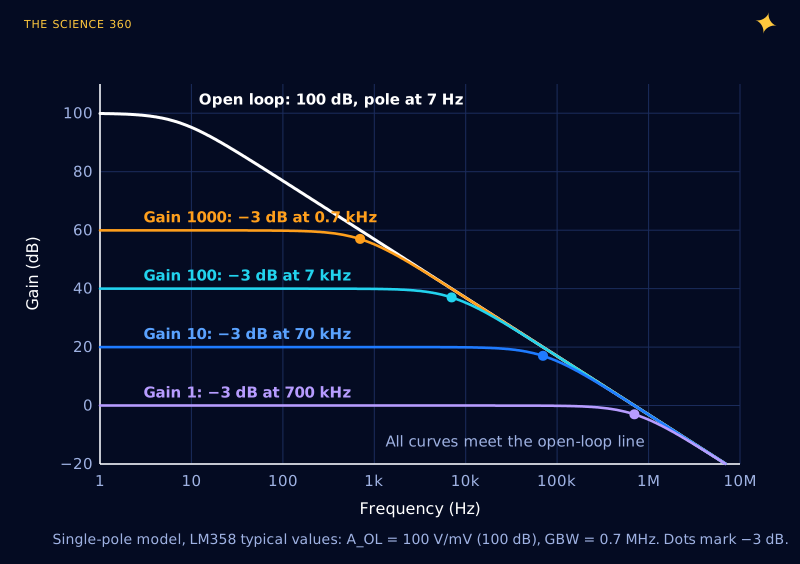
An op amp on its own has enormous gain at DC. TI's LM358 datasheet (revision of October 2024) lists a typical open-loop gain of 100 V/mV, which is 100,000, or 100 dB. That gain does not last. Almost every general-purpose op amp is deliberately built with one dominant pole, a built-in low-pass filter, so that its gain falls at a steady 20 dB per decade over most of its range. A falling line with that slope has a simple property: gain times frequency is the same everywhere on it.

LM358, typical values from the TI datasheet

Open-loop gain A₀, gain bandwidth product GBW and dominant pole f_p:

\begin{aligned}A_0 &= 100\ \mathrm{V/mV} = 10^5\ (100\ \mathrm{dB}) \\ \mathrm{GBW} &= 0.7\ \mathrm{MHz} \\ f_p &= \mathrm{GBW}/A_0 = 700{,}000/100{,}000 \\ &= \mathbf{7\ Hz}\end{aligned}

Check a point on the slope: at 7 kHz the open-loop gain is

0.7\ \mathrm{MHz}/7\ \mathrm{kHz} = 100\ (40\ \mathrm{dB})

So the "amplifier with a gain of 100,000" is an amplifier with a gain of 100,000 only below about 7 Hz. At 1 kHz it is down to 700. That is why you never use an op amp open loop: you wrap feedback around it and trade the excess gain for accuracy and bandwidth.

A quick correction before going on. You will often see the LM358 quoted at "about 1 MHz". TI's current datasheet lists 0.7 MHz typical for the LM358, LM358A and LM2904, and 1.2 MHz for the newer LM358B, along with slew rates of 0.3 and 0.5 V/µs respectively. The round 1 MHz may come from other manufacturers' versions, which I did not check. Whatever the part, read the actual datasheet for the variant you are buying.

Bode plot of LM358 open-loop gain, flat at 100 decibels up to 7 hertz then falling at 20 decibels per decade to 0 decibels at 0.7 megahertz. Closed-loop curves for gains of 1000, 100, 10 and 1 are flat at 60, 40, 20 and 0 decibels and roll off where they meet the open-loop line, at 0.7 kilohertz, 7 kilohertz, 70 kilohertz and 700 kilohertz. — Figure 1. Single-pole model of an LM358 with its typical datasheet values. Each closed-loop response is flat until it runs into the open-loop line, then follows it down. The −3 dB point (dots) is GBW divided by the gain: 0.7 kHz, 7 kHz, 70 kHz and 700 kHz.

Why is the bandwidth GBW divided by the gain?

With feedback fraction β (the share of the output fed back to the inverting input), the closed-loop gain is $A/(1 + A\beta)$ . Where the loop gain $A\beta$ is large, that is just $1/\beta$ . Where it falls toward 1, the op amp has run out of spare gain and the response follows the open-loop line down. The handover happens at the frequency where the open-loop gain equals $1/\beta$ . On a slope where $A = \mathrm{GBW}/f$ , that frequency is:

Closed-loop bandwidth of a single-pole op amp

\begin{aligned}A(f) &\approx \mathrm{GBW}/f\ \ (\text{on the slope}) \\ A &= 1/\beta\ \ \text{at}\ f_c \\ f_c &= \mathrm{GBW} \times \beta = \mathbf{GBW/(1/\beta)}\end{aligned}

$1/\beta$ is the noise gain: $1 + R_f/R_{in}$ for both the inverting and the non-inverting circuit.

Here is the subtlety. In a non-inverting amplifier, the signal gain is $1 + R_f/R_{in}$ , the same as $1/\beta$ , so "divide GBW by the gain" works. In an inverting amplifier the signal gain is $-R_f/R_{in}$ , but the feedback network is identical, so $1/\beta$ is still $1 + R_f/R_{in}$ . The bandwidth follows $1/\beta$ , which is called the noise gain because it is the gain applied to noise (and offset) at the op amp's input. TI's OPA690 datasheet puts it plainly: dividing GBP by the non-inverting signal gain, "also called the noise gain", predicts the closed-loop bandwidth.

Inverting vs non-inverting, LM358 (GBW = 0.7 MHz)

Buffer, gain +1:

\begin{aligned}\text{noise gain} &= 1 \\ \text{bandwidth} &= 0.7\ \mathrm{MHz}/1 \\ &= \mathbf{700\ kHz}\end{aligned}

Inverter, gain −1 (R_f = R_in):

\begin{aligned}\text{noise gain} &= 1 + 1 = 2 \\ \text{bandwidth} &= \mathbf{350\ kHz}\end{aligned}

Non-inverting, gain +10:

\begin{aligned}\text{noise gain} &= 10 \\ \text{bandwidth} &= \mathbf{70\ kHz}\end{aligned}

Inverting, gain −10 ( $R_f/R_{in} = 10$ ):

\begin{aligned}\text{noise gain} &= 11 \\ \text{bandwidth} &= 0.7\ \mathrm{MHz}/11 \\ &= \mathbf{63.6\ kHz}\end{aligned}

Bode plot of signal gain magnitude from 1 kilohertz to 10 megahertz. The non-inverting gain of plus 1 rolls off at 700 kilohertz, the inverting gain of minus 1 at 350 kilohertz. The non-inverting gain of plus 10 rolls off at 70 kilohertz and the inverting gain of minus 10 at 63.6 kilohertz. — Figure 2. Same op amp, same gain magnitudes, different bandwidths. The inverting circuits are always slower because their noise gain is one higher than their signal gain. At gain 10 the difference is 10%; at gain 1 it is a factor of 2.

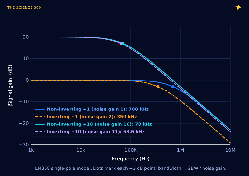
Hugo Coolens made the same point in Electronic Design in 2019 with a 741: open-loop gain 200,000 and open-loop bandwidth 5 Hz, so $\mathrm{GBW} = 1\ \mathrm{MHz}$ . The naive rule predicts 1 MHz for a unity-gain inverter; the right answer is 500 kHz. His general form for the inverting circuit is $(1 + |A_{CL}|) \times \mathrm{BW} = \mathrm{GBW}$ , and he notes the naive version stays within 5% only once the gain is at least about 20.

Noise gain is also why a few circuits surprise people. A summing amplifier with four equal input resistors and the same feedback resistor has a signal gain of −1 from each input, but a noise gain of $1 + 1/(1/4) = 5$ , so its bandwidth is $\mathrm{GBW}/5$ . A transimpedance amplifier for a photodiode has a signal "gain" in ohms, and its stability is set by a noise gain that rises with frequency because of the diode's capacitance.

How much bandwidth do you actually need?

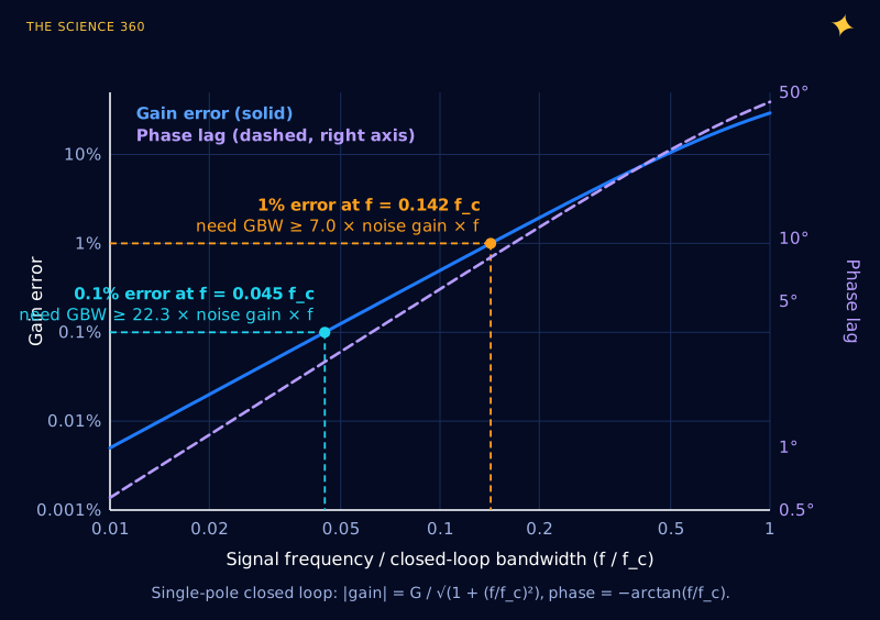
The −3 dB point is where the gain is already 29% low. If you want a gain that is actually accurate, you need to stay well below it. For a single-pole closed loop, the gain falls as $G/\sqrt{1 + (f/f_c)^2}$ and the phase lags by $\arctan(f/f_c)$ .

Design margin for gain accuracy

1% low:

\begin{aligned}1/\sqrt{1 + x^2} &= 0.99 \\ x = f/f_c &= 0.142 \\ \text{need GBW} &\ge \mathbf{7.0 \times \textbf{noise gain} \times f}\end{aligned}

0.1% low:

\begin{aligned}x &= 0.045 \\ \text{need GBW} &\ge \mathbf{22 \times \textbf{noise gain} \times f}\end{aligned}

Example: gain of +10 at 20 kHz (top of the audio band)

LM358:

\begin{aligned}f_c &= 70\ \mathrm{kHz},\ x = 0.286 \\ &\to \text{gain } 3.8\%\ \text{low}\ (-0.34\ \mathrm{dB}) \\ \text{phase lag} &= \mathbf{16^\circ}\end{aligned}

TL072 (GBW 5.25 MHz):

\begin{aligned}f_c &= 525\ \mathrm{kHz},\ x = 0.038 \\ &\to \text{gain } 0.07\%\ \text{low} \\ \text{phase lag} &= \mathbf{2.2^\circ}\end{aligned}

Log-log plot of gain error and phase lag versus signal frequency as a fraction of closed-loop bandwidth, from 0.01 to 1. Gain error rises from 0.005 percent at 0.01 to 29 percent at 1. Marked points: 1 percent error at 0.142 of the bandwidth, requiring gain bandwidth product of at least 7 times noise gain times frequency, and 0.1 percent error at 0.045, requiring 22 times. Phase lag on the right axis rises from about 0.6 degrees to 45 degrees. — Figure 3. Gain error and phase lag of a single-pole closed loop versus how close you are to its bandwidth. Gain error grows as the square of frequency, so it is tiny at first, but phase lag grows linearly and is already 8° at the 1% point. If phase matters, as in active filters, audio crossovers or the anti-noise path in ANC headphones, you need even more margin.

A one-line LM358 preamp with a gain of 100 has a bandwidth of $0.7\ \mathrm{MHz}/100 = 7\ \mathrm{kHz}$ , not good enough for audio even before you think about accuracy. A TL072 at the same gain manages 52.5 kHz. Pick the op amp from the GBW you need, not the GBW printed in the headline of the datasheet.

Is gain bandwidth product always constant?

No, and the place it fails is low gain. Real op amps have more than one pole. The second pole, usually somewhere near the unity-gain frequency, adds phase lag that a single-pole model ignores. At high noise gain the loop crosses over far below that second pole and nothing changes. At low noise gain the loop crosses over close to it, the phase margin shrinks, and the closed-loop response develops a bump before it falls. TI's OPA690 datasheet notes that GBP divided by noise gain "only holds true when the phase margin approaches 90°, as in high-gain configurations."

Generic op amp, GBW = 1 MHz, second pole at 1 MHz

Noise gain 10:

\begin{aligned}\text{phase margin} &= 84^\circ \\ -3\ \mathrm{dB} &\text{ at } 111\ \mathrm{kHz} \\ &(\text{rule says } 100\ \mathrm{kHz})\end{aligned}

Noise gain 2:

\begin{aligned}\text{phase margin} &= 66^\circ \\ -3\ \mathrm{dB} &\text{ at } 707\ \mathrm{kHz} \\ &(\text{rule says } 500\ \mathrm{kHz}) \\ &\text{no peaking}\end{aligned}

Noise gain 1:

\begin{aligned}\text{phase margin} &= 52^\circ \\ \text{peak} &= 1.2\ \mathrm{dB} \\ -3\ \mathrm{dB} &\text{ at } \mathbf{1.27\ MHz} \\ &(\text{rule says } 1\ \mathrm{MHz})\end{aligned}

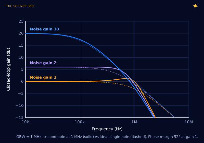
Closed-loop gain versus frequency for an op amp with a 1 megahertz gain bandwidth product and a second pole at 1 megahertz, for noise gains of 10, 2 and 1, compared with dashed single-pole curves. The noise gain 1 curve peaks 1.2 decibels near 800 kilohertz before falling steeply, extending past the single-pole prediction. The noise gain 10 curve matches the single-pole model closely. — Figure 4. Adding a realistic second pole. At noise gain 10 the single-pole rule is nearly exact. At noise gain 1 the response peaks and its −3 dB point moves out, but it then falls at 40 dB per decade. Peaking in frequency means overshoot and ringing in a step response.

Counter-intuitively, the low-gain circuit has more bandwidth than the rule predicts, but it buys it with peaking, overshoot and less stability margin. With a heavier capacitive load the second pole moves down and the bump grows into oscillation. This is the reason some fast op amps are sold as "decompensated", stable only above a minimum noise gain, and why "unity-gain stable" is a specification at all. Current-feedback op amps break the rule more completely: their bandwidth is set mainly by the feedback resistor rather than by the gain.

Source note The current-feedback statement is standard textbook material that I did not check against a source in this session; the Electronic Design article only names current-feedback parts as a case where constant GBW fails.

Why does my op amp distort a sine wave that is well inside its bandwidth?

Because of slew rate, which is a different limit altogether. GBW describes small signals, where everything inside the op amp behaves linearly. Slew rate (SR) is the fastest the output can change, set by how much current the input stage can push into the internal compensation capacitor. Once the output is asked to move faster, the op amp is no longer a linear amplifier: the output just ramps at SR until it catches up.

Full-power bandwidth from slew rate

A sine $V_p \sin(2\pi f t)$ changes fastest at its zero crossings:

dV/dt = 2\pi f V_p

Largest undistorted frequency:

f_{\max} = \mathrm{SR}/(2\pi V_p)

LM358, SR = 0.3 V/µs, V_p = 10 V:

\begin{aligned}f_{\max} &= 300{,}000/(2\pi \times 10) \\ &= \mathbf{4.8\ kHz}\end{aligned}

Same chip at V_p = 1 V: 47.7 kHz.

LM358B (0.5 V/µs) at 10 V: 8.0 kHz. TL072 (20 V/µs) at 10 V: 318 kHz.

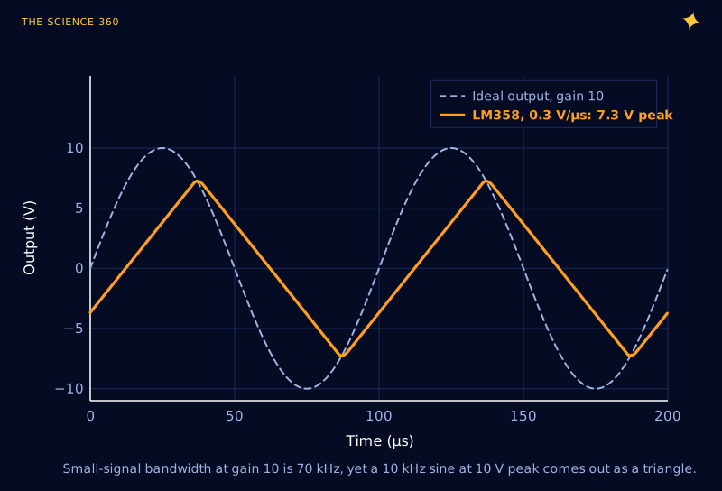
Time plot over 200 microseconds of an ideal 10 kilohertz, 10 volt peak sine wave in dashed grey and the LM358 output in orange. The output is a triangle wave ramping at 0.3 volts per microsecond, lagging the ideal sine and reaching only 7.3 volts peak. — Figure 5. Simulated LM358 at a gain of 10, asked for 10 kHz at 10 V peak. Its small-signal bandwidth at this gain is 70 kHz, seven times higher than the signal, but at 0.3 V/µs the output can only ramp, producing a lagging triangle of 7.3 V peak. Turn the amplitude down below about 4.8 V and the sine comes back.

There is a neat way to see where the two limits cross. In the linear regime an output step ΔV settles exponentially with time constant $1/(2\pi f_c)$ , so its initial rate of change is $2\pi f_c \Delta V$ . That exceeds the slew rate when $\Delta V > \mathrm{SR}/(2\pi f_c)$ .

Largest step that stays linear, LM358 at gain +10

\begin{aligned}f_c &= 70\ \mathrm{kHz} \\ 2\pi f_c &= 4.4 \times 10^5\ \mathrm{s^{-1}} \\ \Delta V_{\max} &= \frac{0.3\ \mathrm{V/\mu s}}{4.4 \times 10^5\ \mathrm{s^{-1}}} \\ &= \frac{0.3 \times 10^6}{4.4 \times 10^5} = \mathbf{0.68\ V}\end{aligned}

Any output step bigger than about 0.7 V is slew-limited, not bandwidth-limited.

That is why "the scope shows a triangle" and "the frequency response looks fine on a small test signal" are both common reports about the same circuit. The fix is either a faster op amp or a smaller swing. When you are filtering a slow sensor signal, as in an RC time-constant problem, neither limit matters much; when you are driving a 10 V audio line, both do.

A checklist for choosing an op amp by bandwidth

Work out the noise gain, $1 + R_f/R_{in}$ (or the effective version for summing and transimpedance circuits). Multiply it by the highest signal frequency and by 7 for 1% accuracy, or 22 for 0.1%: that is your minimum GBW. Compute $2\pi f V_p$ for your largest swing and compare it with the slew rate, with margin, because both numbers on the datasheet are typical values. If your noise gain is close to 1 or you are driving capacitance, look at the phase margin or the small-signal step response plots rather than GBW alone. And if the op amp is buffering a reference or feeding an ADC, remember that its output impedance rises with frequency as the loop gain falls, which is where a local decoupling capacitor earns its place.

Rules of thumb:

\text{bandwidth} = \mathrm{GBW}/\text{noise gain}

; an inverter of gain

-G

has noise gain

G + 1

; 1% accuracy needs

\mathrm{GBW} \ge 7 \times \text{noise gain} \times f

; slew-limited above

f = \mathrm{SR}/(2\pi V_p)

; the single-pole rule is optimistic about stability and slightly pessimistic about bandwidth at noise gains below about 3.

FAQ

What is the gain bandwidth product of an op amp?

For most voltage-feedback op amps the open-loop gain falls at 20 dB per decade over a wide range, so gain times frequency is constant along that slope. That constant is the gain bandwidth product. In a feedback circuit the closed-loop bandwidth is roughly the gain bandwidth product divided by the circuit's noise gain.

Why does an inverting amplifier with gain -1 have half the bandwidth?

Bandwidth depends on the noise gain, $1 + R_f/R_{in}$ , which is the gain the op amp applies to a signal at its non-inverting input. A gain of −1 uses equal resistors, so its noise gain is 2 and its bandwidth is half the gain bandwidth product, while a +1 buffer has noise gain 1 and the full bandwidth.

Is slew rate the same as bandwidth?

No. Gain bandwidth product limits small signals; slew rate is the fastest the output voltage can change, and it limits large signals. A sine of peak voltage $V_p$ needs a slew rate of $2\pi f V_p$ . An LM358 at 0.3 V per microsecond can only deliver a 10 V peak sine up to about 4.8 kHz, even though its small-signal bandwidth at gain 10 is 70 kHz.

What is the gain bandwidth product of the LM358?

Texas Instruments' current LM358 datasheet lists a typical gain bandwidth product of 0.7 MHz and a slew rate of 0.3 V per microsecond for the LM358 and LM358A. The newer LM358B is listed at 1.2 MHz and 0.5 V per microsecond. Typical values vary between parts, so leave margin.

How much gain bandwidth product do I need?

To keep a single-pole amplifier's gain error below 1 percent at frequency f, you need a gain bandwidth product of at least about 7 times the noise gain times f. For 0.1 percent you need about 22 times. Then check slew rate separately, using $2\pi f V_p$ for your largest output swing.

Sources

Texas Instruments, LM358, LM358A, LM358B, LM2904 datasheet, SLOS068AB, revised October 2024 (GBW 0.7 MHz and SR 0.3 V/µs for LM358; 1.2 MHz and 0.5 V/µs for LM358B; A_OL 100 V/mV typ): ti.com/lit/ds/symlink/lm358.pdf
Texas Instruments, TL07x datasheet, SLOS080W, revised July 2025 (GBW 5.25 MHz, 3 MHz for NS/PS packages and M grade; SR 20 V/µs typ): ti.com/lit/ds/symlink/tl072.pdf
Texas Instruments, OPA690 datasheet (GBP divided by noise gain; holds when phase margin approaches 90°): ti.com/product/OPA690
H. Coolens, "Gain-Bandwidth Product is Not (Always) Constant", Electronic Design, April 2019: electronicdesign.com

Method note: all frequency responses are computed from single-pole (and, in Figure 4, two-pole) transfer functions using the datasheet typical values. Figure 5 integrates a first-order closed loop with a hard slew-rate clamp. Real parts vary with supply voltage, load and temperature, and typical values are not guaranteed.

Header image: NASA (image iss018e027439), regraded for this article.