How Does a Load Cell Work? Strain Gauges and the HX711 • The Science 360

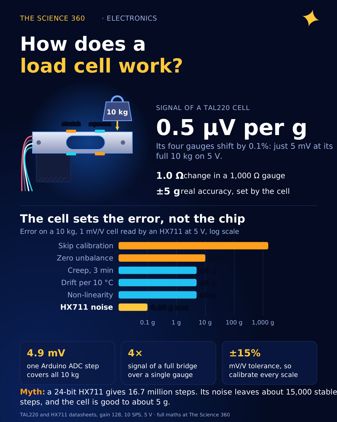
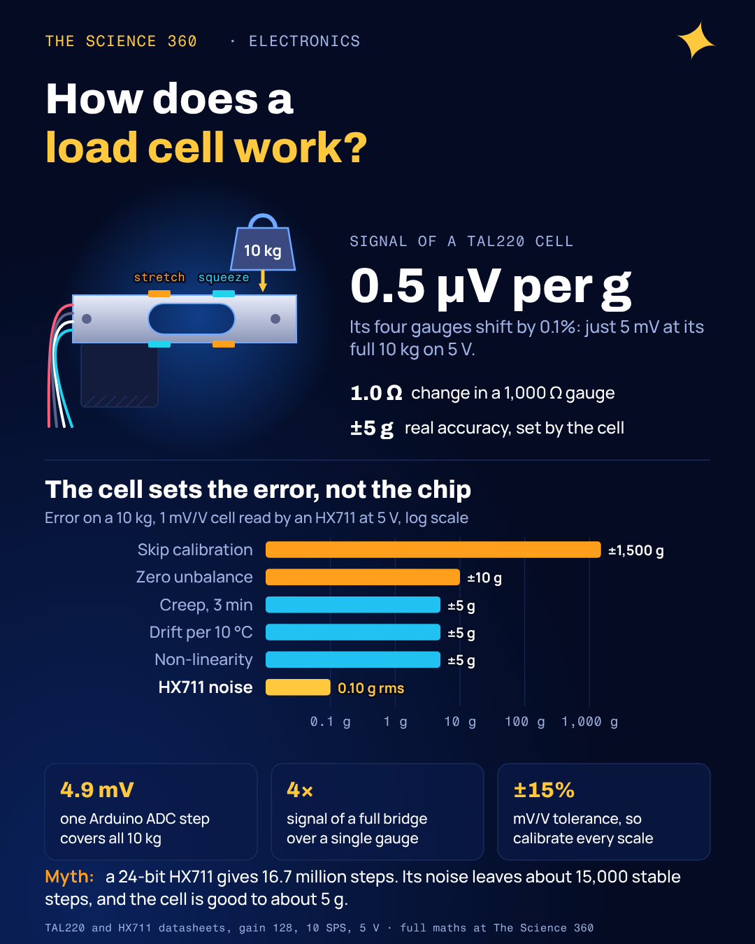
Put 10 kg on a common bar-type load cell and its aluminium body shortens and stretches by about 500 millionths. The four foil gauges glued to it change resistance by 1 Ω out of 1,000 Ω. The signal that comes out of the four wires is 5 mV when excited at 5 V, or half a microvolt for each gram. Everything about how a cheap kitchen scale manages to read to the gram follows from that one fact: the signal is tiny, and every design choice in the cell and in the HX711 chip exists to keep it clean.

The pages that rank for this question describe the parts (spring element, strain gauge, Wheatstone bridge) but almost never put numbers on them. Without numbers you cannot answer the questions people actually have: why the HX711's 24 bits do not give you 16 million steps, why a reading drifts by grams over a few minutes, and why calibration is not optional. This post follows the signal from the metal to the microcontroller, with figures from the TAL220 cell datasheet and the HX711 datasheet.

Quick answerA load cell is a metal spring carrying four strain gauges. Under load two gauges stretch and two compress, changing resistance by about 0.1%. Wired as a Wheatstone bridge they give an output proportional to force, typically 1 to 2 mV per volt of excitation at full load: 5 mV for a 1 mV/V cell on 5 V.

Infographic: How does a load cell work? A bar load cell with a binocular hole is bolted at one end and loaded with 10 kg at the other, with four strain gauges on its webs and four coloured wires. A 10 kg, 1 mV/V cell on 5 V gives just 0.5 microvolts per gram: each 1,000 ohm gauge changes by 1 ohm. A log-scale bar chart of errors shows skipping calibration at ±1,500 g, zero unbalance ±10 g, creep, temperature drift and non-linearity ±5 g each, and HX711 noise only 0.10 g rms. Tiles: one Arduino ADC step is 4.9 mV, a full bridge gives 4 times a single gauge's signal, and the ±15% tolerance makes calibration mandatory. — Tap the image to view it full size. View the accessible, editable SVG.

The spring element: a load cell is a very stiff spring

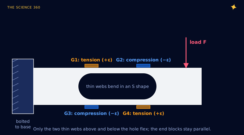
The weight does not press on a sensor. It bends a precisely machined piece of metal, and the sensor reads the bend. The common bar cell in hobby scales (the TAL220 and its many clones) is a parallel beam: a rectangular aluminium bar with a binocular hole cut through the middle, bolted down at one end and loaded at the other. The hole leaves two thin webs, one above and one below. Under load the free end drops while staying parallel, so each web bends into a shallow S, stretching its surface at one end and squeezing it at the other.

Side view of a parallel beam load cell. The left end is bolted to a base and a downward load F acts near the right end. A rounded binocular hole through the middle leaves two thin webs. Strain gauge G1 on the top surface above the left end of the hole is in tension, G2 above the right end is in compression, G3 below the left end is in compression and G4 below the right end is in tension. — Figure 1. Gauge positions on a parallel beam load cell. The webs bend in an S shape, so each surface has a tension zone and a compression zone. Placing gauges at both ends of both webs gives two in tension and two in compression.

How much does it bend? Micro-Measurements, one of the main strain gauge makers, says that "most load cells and transducers are manufactured so the full-scale rated mechanical load will produce 1000 µɛ at the gage locations." A microstrain (µε) is a length change of one part per million. A 1 mV/V cell like the TAL220 works out to about 500 µε at its gauges, as we show below. In aluminium that is a surface stress of roughly 35 MPa, a small fraction of what the alloy can take, which is why the cell is rated for 120% safe overload and 150% ultimate overload.

Strain at rated load (TAL220-class cell, our estimate):

\begin{aligned}\varepsilon &\approx 500\ \mu\varepsilon = 0.0005 \\ \text{stress } \sigma &= E \times \varepsilon \\ &\approx 69\ \mathrm{GPa} \times 0.0005 \\ &\approx \mathbf{35\ MPa}\ \text{(aluminium)}\end{aligned}

Over a 6 mm gauge grid:

\begin{aligned}\text{length change} &= 6\ \mathrm{mm} \times 0.0005 \\ &= \mathbf{3\ \mu m}\end{aligned}

Source note The TAL220 datasheet does not give the strain at the gauges or the alloy. The 500 µε figure is inferred from its 1.0 mV/V rating with a gauge factor of 2 and a full four-arm bridge. Young's modulus of 69 GPa is a typical handbook value for aluminium alloys, and the 6 mm grid length is illustrative; I did not check either against a source for this specific cell.

How a strain gauge turns stretch into resistance

A foil strain gauge is a zigzag of thin metal track on a plastic backing, glued to the spring. Stretch it and the track gets longer and thinner, so its resistance rises; compress it and resistance falls. The ratio of fractional resistance change to strain is the gauge factor:

\text{GF} = \frac{\Delta R/R}{\varepsilon}

HBM: $\text{GF} \approx 2.0$ for constantan, $\approx 2.2$ for Modco foils.

At 500 µε:

\begin{aligned}\Delta R/R &= 2.0 \times 0.0005 \\ &= 0.001 = \mathbf{0.1\%}\end{aligned}

On a 1,000 Ω gauge:

\Delta R = \mathbf{1.0\ \Omega}

About 1.0 of that 2.0 is pure geometry: a stretched wire of fixed volume gets longer and thinner, and resistance goes as length over area. The rest is a change in the alloy's resistivity under strain. Semiconductor gauges have far higher gauge factors, but foil gauges are used in nearly every load cell because their response is linear and stable.

A 0.1% change is the crux. A temperature change of a few degrees shifts the resistance of most metals by a comparable amount, and the wire from your scale to your board has resistance of the same order as ΔR. Measuring 1 Ω in 1,000 Ω directly with an ohmmeter is hopeless. You need a circuit that ignores the 1,000 Ω and sees only the change.

Why load cells use a Wheatstone bridge

A Wheatstone bridge is two voltage dividers side by side, fed from the same excitation voltage, with the output taken between their midpoints. When all four arms are equal, both midpoints sit at exactly half the excitation and the output is zero, regardless of the absolute resistance. Only imbalance shows up. It is the same divider arithmetic as a voltage divider or a thermistor divider, done twice and subtracted.

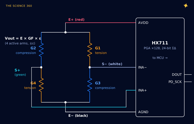
Schematic of a load cell full bridge wired to an HX711. HX711 AVDD drives the E plus red wire to the top of both bridge halves; E minus black goes to AGND. The left half has G2 in compression on top and G4 in tension below, with their midpoint S plus green to INA plus. The right half has G1 in tension on top and G3 in compression below, with the midpoint S minus white to INA minus. DOUT and PD_SCK go to the microcontroller. — Figure 2. A four-active-arm bridge on an HX711, using the TAL220's wire colours. Tension gauges sit in diagonally opposite arms, so when the load arrives S+ rises and S− falls, and their effects add.

With all four gauges active, two going up by ΔR and two going down by ΔR in the right arms, the output is exactly linear:

\begin{aligned}V(S{+}) &= E \times \frac{R + \Delta R}{2R} \\ V(S{-}) &= E \times \frac{R - \Delta R}{2R} \\ V_{\mathrm{out}} &= V(S{+}) - V(S{-}) \\ &= E \times \Delta R/R \\ &= \mathbf{E \times GF \times \varepsilon}\end{aligned}

TAL220: $\text{GF} \times \varepsilon = 0.001$ → 1.0 mV/V (its rated output)

At 5 V excitation, full 10 kg:

\begin{aligned}V_{\mathrm{out}} &= 5\ \mathrm{V} \times 0.001 = \mathbf{5.0\ mV} \\ \text{per gram} &= 5.0\ \mathrm{mV}/10{,}000\ \mathrm{g} \\ &= \mathbf{0.5\ \mu V/g}\end{aligned}

Micro-Measurements writes the same rule as 0.5 µV/V per microstrain for each active arm with a gauge factor of 2. Four arms at 1,000 µε give their 2 mV/V example; our 500 µε gives 1 mV/V.

Figure 3. Output per volt of excitation for quarter, half and full bridges (our calculation,

\text{GF} = 2.0

). The full bridge gives four times the signal of a single gauge, and is exactly linear when its arms change by equal and opposite amounts.

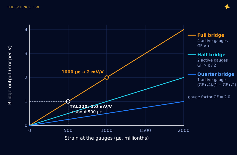
Signal size is only half of why the full bridge wins. The other half is temperature. All four gauges are the same alloy on the same piece of metal, so a temperature change moves all four resistances together. In a balanced bridge an equal change in every arm cancels exactly; only the opposite changes from strain survive. A single gauge (a quarter bridge) has no such partner, and its output is also slightly non-linear: $(\text{GF}\,\varepsilon/4)/(1 + \text{GF}\,\varepsilon/2)$ , which is 0.1% low at 1,000 µε. The bridge also makes the output ratiometric: it is a fraction of the excitation, so if you measure it with an ADC whose reference is that same excitation, supply drift cancels out.

What the HX711 does with 5 millivolts

Five millivolts full scale is too small for a microcontroller ADC: on a 10-bit, 5 V Arduino one count is 4.9 mV, so the entire 10 kg range would be one count. The HX711 is a 24-bit sigma-delta converter with a low-noise programmable gain amplifier in front, built for exactly this job. Its channel A has gain 128 or 64, and the datasheet gives the full-scale input as $\pm 0.5 \times \text{AVDD}/\text{gain}$ :

Gain 128, $\text{AVDD} = 5\ \mathrm{V}$ :

\begin{aligned}\text{full scale} &= \pm 0.5 \times 5/128 \\ &= \mathbf{\pm 19.5\ mV}\end{aligned}

(the datasheet rounds to ±20 mV). In bridge terms:

0.5/128 = \mathbf{3.91\ mV/V}

independent of AVDD (ratiometric).

\begin{aligned}\text{one count} &= 39.06\ \mathrm{mV}/2^{24} \\ &= \mathbf{2.33\ nV}\end{aligned}

TAL220 full load:

\begin{aligned}&5.0\ \mathrm{mV}/2.33\ \mathrm{nV} \\ &= \mathbf{2{,}147{,}484\ counts}\end{aligned}

Per count:

\begin{aligned}&10{,}000\ \mathrm{g}/2{,}147{,}484 \\ &= 0.0047\ \mathrm{g}\end{aligned}

A 1 mV/V cell uses only about a quarter of the HX711's positive range, a 2 mV/V cell about half. That is fine: the range above full load is headroom for overload and zero offset. Check the common-mode limit too. The bridge outputs sit at about $\text{AVDD}/2$ (2.5 V at 5 V), and the HX711 needs its inputs between $\text{AGND} + 1.2\ \mathrm{V}$ and $\text{AVDD} - 1.3\ \mathrm{V}$ , a 1.2 to 3.7 V window at 5 V. On a 2.7 V supply that window narrows to 1.2 to 1.4 V around a 1.35 V bridge midpoint, which still works but with little margin.

Is the HX711 really 24-bit? Counts versus noise

This is the misconception page one never touches. The 0.0047 g per count above is not your resolution. The converter's own noise is many counts wide, and noise sets what you can actually resolve. The HX711 datasheet gives input-referred noise at gain 128 of 50 nV rms at 10 samples per second and 90 nV rms at 80 SPS:

10 SPS:

\begin{aligned}\text{noise} &= 50\ \mathrm{nV\ rms} = 50/2.33 \\ &= \mathbf{21\ counts\ rms} \\ \text{in grams} &= 50\ \mathrm{nV}/0.5\ \mu\mathrm{V\ per\ g} \\ &= \mathbf{0.10\ g\ rms} \\ \text{peak-to-peak} &= 330\ \mathrm{nV} = \mathbf{0.66\ g}\end{aligned}

(peak-to-peak uses the usual 6.6 × rms convention)

\begin{aligned}\text{effective} &= \log_2(5\ \mathrm{mV}/50\ \mathrm{nV}) \\ &= \log_2(100{,}000) = \mathbf{16.6\ bits} \\ \text{noise-free} &= \log_2(5\ \mathrm{mV}/330\ \mathrm{nV}) \\ &= \log_2(15{,}150) = \mathbf{13.9\ bits}\end{aligned}

80 SPS: 90 nV rms → 0.18 g rms, 1.19 g peak-to-peak, 13.0 noise-free bits

Averaging 10 readings at 10 SPS (1 second), if the noise is white:

0.10/\sqrt{10} = \mathbf{0.03\ g\ rms}

So the honest description of an HX711 with a 1 mV/V, 10 kg cell is "about 15,000 stable steps across full scale", not "16.7 million". That is still excellent, and it is why a 10 kg scale can show whole grams without flicker. But 24 bits is the width of the output word, not the information in it. The distinction between resolution, noise and accuracy is the whole subject of ADC resolution vs accuracy, and the $\sqrt{N}$ averaging gain only holds while the noise is random; low-frequency drift does not average away.

Two side notes on data rate. The 10 SPS mode is quieter and, per the datasheet, rejects 50 and 60 Hz mains pickup simultaneously; the 80 SPS mode doubles the noise for an eightfold faster update. If your readings show a slow wobble, mains interference from long unshielded wires is a likely cause, see ground loop hum and why mains is 50 or 60 Hz.

Source note The noise figures are datasheet typical values measured by Avia under its own conditions, presumably at AVDD = 5 V. Many hobby HX711 modules regulate AVDD lower than 5 V (the datasheet requires the regulator output to sit at least 100 mV below VSUP), which shrinks the bridge signal while the input-referred noise stays similar, and their layouts are not the reference design. Clone modules may measure noisier than the numbers above; I did not test one.

Where load cell errors really come from

Here is the twist. Once the HX711 has given you 0.1 g of noise, almost every remaining error comes from the load cell itself. The TAL220 datasheet lists, as a percentage of full scale (FS = 10 kg here):

TAL220 specification	Value	On a 10 kg cell
Rated output	1.0 ± 0.15 mV/V	±1,500 g at full load if not calibrated
Zero unbalance	±0.1% FS	±10 g (removed by tare)
Non-linearity	±0.05% FS	±5 g
Hysteresis	±0.05% FS	±5 g
Repeatability	±0.03% FS	±3 g
Creep	±0.05% FS per 3 min	±5 g
Temperature effect on zero	±0.05% FS per 10 °C	±5 g per 10 °C
Temperature effect on span	±0.05% FS per 10 °C	±5 g per 10 °C at full load
Combined error	±0.05% FS	±5 g

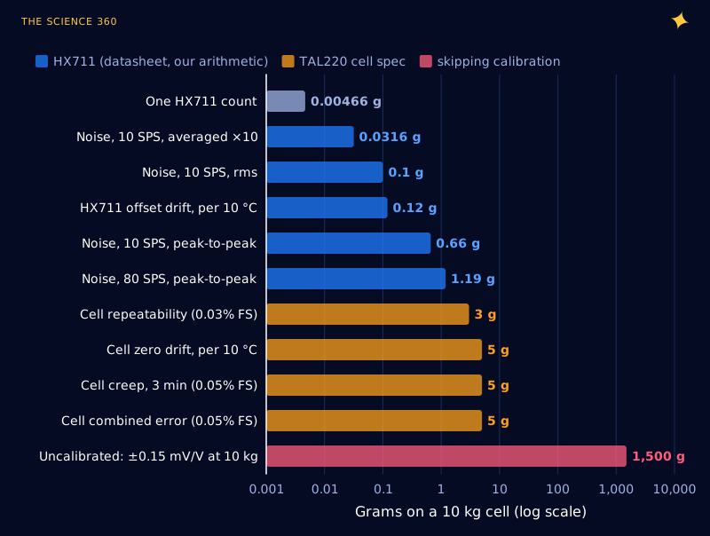
Figure 4. Error budget for a 10 kg cell on an HX711 at gain 128, 5 V (our arithmetic from the two datasheets). The electronics are one to two orders of magnitude better than the cell; skipping calibration is three orders worse.

Compare the electronics. The HX711 offset drift is ±6 nV/°C at gain 128, which against our 0.5 µV per gram is 0.012 g/°C, or 0.12 g per 10 °C: forty times smaller than the cell's own zero drift. Its gain drift of ±5 ppm/°C is 0.5 g per 10 °C at full load. In other words, a 24-bit ADC on a 0.05% load cell is like a micrometer on a rubber ruler. The readings are steady to a tenth of a gram, and correct to about 5 g.

Creep is the error people notice. Leave a heavy object on the scale and the reading slowly rises by a few grams over minutes, as the metal and the gauge adhesive relax. The fix is procedural: tare immediately before a measurement, read soon after the load settles, and do not use a hobby cell for long-term weight logging without expecting drift.

How to calibrate an HX711 scale: a worked example

Calibration handles the two big unknowns: zero offset (the cell is never perfectly balanced) and the true sensitivity (anywhere from 0.85 to 1.15 mV/V for a TAL220). Two readings fix both. Suppose this particular cell is really 1.07 mV/V:

Step 1, empty scale (tare): $\text{raw} = \mathbf{1{,}379}$ (average of 10 readings)

Step 2, 1,000.0 g reference mass: $\text{raw} = \mathbf{231{,}160}$

\begin{aligned}\text{scale factor} &= \frac{231{,}160 - 1{,}379}{1{,}000.0\ \mathrm{g}} \\ &= \mathbf{229.78\ counts\ per\ gram}\end{aligned}

Check:

\begin{aligned}229.78 \times 10{,}000\ \mathrm{g} &= 2{,}297{,}800\ \text{counts} \\ &= 1.07 \times 2{,}147{,}484\end{aligned}

at full load, so the cell is 1.07 mV/V.

Step 3, unknown object: $\text{raw} = 116{,}270$

\frac{116{,}270 - 1{,}379}{229.78} = \mathbf{500.0\ g}

// HX711 on pins DOUT = 3, SCK = 2 (bit-banged, gain 128, channel A)
long readRaw() {
  while (digitalRead(3) == HIGH) {}           // wait for data ready
  long v = 0;
  for (int i = 0; i < 24; i++) {
    digitalWrite(2, HIGH); delayMicroseconds(1);
    v = (v << 1) | digitalRead(3);
    digitalWrite(2, LOW);  delayMicroseconds(1);
  }
  digitalWrite(2, HIGH); delayMicroseconds(1); // 25th pulse: next = ch A, gain 128
  digitalWrite(2, LOW);
  if (v & 0x800000) v |= 0xFF000000;           // sign-extend 24-bit two's complement
  return v;
}
// grams = (readRaw()-OFFSET) / 229.78

The pulse count matters: the HX711 datasheet sets the next conversion's channel and gain by the number of clock pulses, 25 for channel A at gain 128, 26 for channel B at 32, 27 for channel A at 64. Holding PD_SCK high for more than 60 µs powers the chip down, so do not let an interrupt stretch a clock pulse. Choose a reference mass near the top of your working range, because any error in the reference scales every reading, and a heavy reference makes the counts-per-gram estimate less sensitive to noise. If the scale must be accurate across temperature, calibrate at the temperature you will use it, since span drift is ±0.05% per 10 °C.

Practical wiring that keeps the microvolts clean

Mount the cell as designed: bolt the fixed end to a rigid base and load only the free end, through the arrow direction marked on the body. Any load path that shortcuts the webs (a platform touching the base, an overtightened screw) changes the sensitivity.
Keep the four wires short and twisted together, away from motor and mains wiring. The bridge output impedance is 1,000 Ω, so it picks up interference easily.
Give the HX711 its own clean supply rail and a local decoupling capacitor; the datasheet's application circuit also places 10 µF on AVDD and 0.1 µF on VBG.
Remember the excitation current: a 1,000 Ω bridge draws 5 mA at 5 V, more than the HX711 itself (1.4 mA analog). On batteries, use the PD_SCK power-down between readings.
Expect the signal you calculated. If a 10 kg, 1 mV/V cell at 5 V reads far more than about 2.1 million counts at full load, or the reading rails at 0x7FFFFF, check for a swapped wire or a damaged gauge before blaming the code.

The short version for your bench: a load cell is a spring whose four gauges change by about 0.1% at full load; the full Wheatstone bridge turns that into 1 to 2 mV per volt and cancels temperature. With a 1 mV/V cell on 5 V, the HX711 at gain 128 sees 5 mV over 2.1 million counts but resolves about 15,000 noise-free steps (0.1 g rms on 10 kg). The cell's own creep, drift and non-linearity, about 5 g each, set the real accuracy, and the ±15% tolerance on mV/V makes calibration mandatory.

FAQ

How does a load cell work?

A metal spring element bends slightly under load. Four strain gauges bonded to it change resistance by about 0.1% at full load, two up and two down, and a Wheatstone bridge turns that into a voltage proportional to force: typically 1 to 2 mV per volt of excitation at rated load.

What does 1 mV/V mean on a load cell?

It is the bridge output at rated load per volt of excitation. A 1 mV/V, 10 kg cell excited at 5 V gives 5 mV at 10 kg, or 0.5 µV per gram. The rating usually has a tolerance of around ±15%, so every scale must be calibrated with a known mass.

What resolution does an HX711 really give?

Far less than 24 bits. At gain 128 and 10 samples per second the datasheet input noise is 50 nV rms. With a 1 mV/V cell on 5 V that is about 16.6 effective bits and about 14 noise-free bits, or 0.1 g rms on a 10 kg cell, against 2.1 million counts of nominal span.

Why does my load cell reading drift?

Mostly the cell, not the HX711. A typical TAL220 cell specifies zero drift of 0.05% of full scale per 10 °C and creep of 0.05% in 3 minutes, which is 5 g each on a 10 kg cell. The HX711's offset drift adds only about 0.012 g per degree on the same setup.

How do I calibrate an HX711 load cell?

Read the raw value empty (the offset), then with a known reference mass, and divide the difference by that mass to get counts per gram. Weight is then (raw minus offset) divided by counts per gram. Use a reference near the top of your range and re-tare often to remove zero drift.

Sources

Avia Semiconductor, HX711 24-bit ADC for weigh scales datasheet (full scale $\pm 0.5\,\text{AVDD}/\text{gain}$ , ±20 mV at gain 128 and 5 V, input noise 50 nV rms at 10 SPS and 90 nV at 80 SPS, offset drift ±6 nV/°C, gain drift ±5 ppm/°C, common mode $\text{AGND} + 1.2\ \mathrm{V}$ to $\text{AVDD} - 1.3\ \mathrm{V}$ , 50 and 60 Hz rejection, 25/26/27 pulse gain selection, 60 µs power-down, regulator $V_{\mathrm{AVDD}} = V_{\mathrm{BG}}(R_1 + R_2)/R_1$ at least 100 mV below VSUP, 1.4 mA analog current): cdn.sparkfun.com HX711 datasheet PDF
HTC Sensor, TAL220 parallel beam load cell datasheet (rated output 1.0 ± 0.15 mV/V, 5 to 10 V excitation, 1,000 Ω input and output resistance, non-linearity, hysteresis, creep, zero and span temperature coefficients, combined error, overload ratings, wire colours): cdn.sparkfun.com TAL220 datasheet PDF
Micro-Measurements strain blog, "Strain Gage Output" (0.5 µV/V per µε per active arm at GF 2.0; most transducers designed for 1,000 µε at rated load; 2 mV/V example): strainblog.micro-measurements.com/node/56
HBM, Technical Note TN022, "Gauge Factor Deviation" (gauge factor about 2.0 for constantan and 2.2 for Modco): hbm.com TN022 PDF

Method note: Figure 3 and the error budget in Figure 4 are our own calculations from the cited datasheets. The calibration readings are an illustrative example, not a measurement.

Header image: NASA/Radislav Sinyak (image jsc2022e045769), regraded for this article.

The spring element: a load cell is a very stiff spring

How a strain gauge turns stretch into resistance

Why load cells use a Wheatstone bridge

What the HX711 does with 5 millivolts

Is the HX711 really 24-bit? Counts versus noise

Where load cell errors really come from

How to calibrate an HX711 scale: a worked example

Practical wiring that keeps the microvolts clean

FAQ

How does a load cell work?

What does 1 mV/V mean on a load cell?

What resolution does an HX711 really give?

Why does my load cell reading drift?

How do I calibrate an HX711 load cell?

Related on The Science 360

Sources