What Is VSWR? Reflections, Return Loss and Real Loss • The Science 360

Q: How do you convert VSWR to return loss?

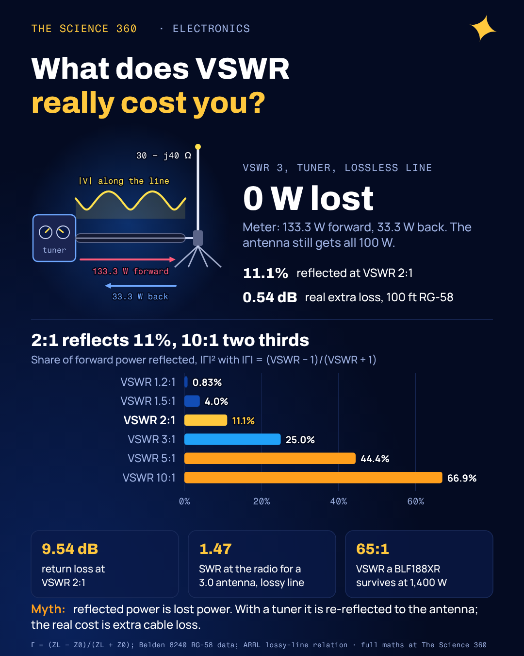
Put an inline wattmeter between a 100 W transmitter with an antenna tuner and an antenna that presents $30 - j40\ \Omega$ , and the meter reads 133.3 W forward and 33.3 W reflected. Most people's first reaction is that a quarter of their power is bouncing back and cooking the radio. On a low-loss feedline the antenna is in fact receiving the full 100 W. The 33 W is real, it is travelling backwards, and it is not lost.

That gap between "reflected" and "lost" is where most explanations of VSWR go soft. The glossary entries on page one of Google define the ratio and stop, or print a table saying VSWR 2:1 "loses" 11% of the power without saying when that is true. Here we build VSWR from the reflection coefficient, convert it with worked numbers, and then follow the reflected power to see what it actually costs.

Quick answerVSWR (voltage standing wave ratio) is the ratio of the highest to the lowest RMS voltage along a transmission line, set by how badly the load mismatches the line:

\text{VSWR} = (1 + |\Gamma|)/(1 - |\Gamma|)

. VSWR 2:1 means 11% of the forward power is reflected. Whether that power is lost depends on the feedline loss and the source, not on VSWR alone.

Infographic: What does VSWR really cost you? A drawing shows a radio and tuner feeding coax to a vertical antenna of 30 minus j40 ohms, with the standing wave along the line and 133.3 W forward and 33.3 W reflected. With a tuner on a lossless line no power is lost and the antenna gets all 100 W; on 100 ft of RG-58 at 10 MHz the mismatch costs an extra 0.54 dB. A bar chart of reflected power shows 0.83% at VSWR 1.2, 4.0% at 1.5, 11.1% at 2, 25.0% at 3, 44.4% at 5 and 66.9% at 10. Tiles: 9.54 dB return loss at VSWR 2; a lossy line makes a 3.0 antenna read 1.47 at the radio. — Tap the image to view it full size. View the accessible, editable SVG.

What does VSWR actually measure?

A transmission line such as coax has a characteristic impedance Z₀, 50 Ω for most RF gear (the reason for 50 Ω coax is a compromise between loss and power handling). A wave travelling down the line carries voltage and current in the fixed ratio Z₀. When it reaches a load whose impedance Z_L is not Z₀, the load cannot satisfy both the wave's V/I ratio and its own, so part of the wave is sent back. The fraction, in amplitude and phase, is the reflection coefficient:

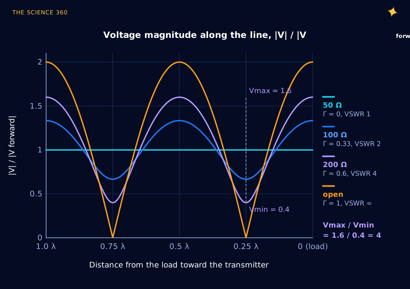
\begin{aligned}\Gamma &= \frac{Z_L - Z_0}{Z_L + Z_0} \\ \text{fraction of power reflected} &= |\Gamma|^2\end{aligned}

The forward and reflected waves now share the same cable. Where their phases line up the voltages add, and a quarter wavelength away they subtract. The result is a stationary pattern of voltage peaks and troughs, the standing wave. Its peak is $|V_{\mathrm{fwd}}|(1 + |\Gamma|)$ and its trough is $|V_{\mathrm{fwd}}|(1 - |\Gamma|)$ , so the ratio of the two depends only on |Γ|:

\begin{aligned}\text{VSWR} &= V_{\max}/V_{\min} \\ &= \frac{1 + |\Gamma|}{1 - |\Gamma|}\end{aligned}

Inverse:

|\Gamma| = \frac{\text{VSWR} - 1}{\text{VSWR} + 1}

Figure 1 plots the pattern for a few resistive loads. A matched 50 Ω load gives a flat line. A 100 Ω load gives a ripple between 0.67 and 1.33 times the forward voltage, a ratio of 2. An open circuit reflects everything and the voltage swings between zero and twice the forward value. The peaks repeat every half wavelength, which is why VSWR is quoted as one number for the whole line: on a lossless line the ratio is the same wherever you stand.

Plot of normalized voltage magnitude along a 50 ohm line versus distance from the load, from 0 to 1 wavelength. A 50 ohm load gives a flat line at 1. A 100 ohm load ripples between 0.67 and 1.33 (VSWR 2). A 200 ohm load ripples between 0.4 and 1.6 (VSWR 4). An open circuit swings between 0 and 2. Peaks repeat every half wavelength. — Figure 1. Voltage magnitude along a lossless 50 Ω line, computed from $|V| = |V_{\mathrm{fwd}}| \times |1 + \Gamma e^{-j2\beta d}|$ . The load sits at the right. Resistive loads above 50 Ω put a voltage peak at the load; the open circuit is the limiting case.

How to calculate Γ, VSWR and return loss from an impedance

Three quantities describe the same mismatch, and engineers in different corners of the field prefer different ones. Antenna people and radio amateurs quote VSWR. Network analyzer users quote return loss. Circuit designers work in Γ, which keeps the phase. Here is one complex load carried through all of them.

Worked example: an antenna that measures $30 - j40\ \Omega$ on a 50 Ω line. This is a plausible feedpoint impedance for an antenna cut slightly short, which looks capacitive.

\begin{aligned}\Gamma &= \frac{30 - j40 - 50}{30 - j40 + 50} \\ &= \frac{-20 - j40}{80 - j40} \\ |\text{numerator}| &= \sqrt{20^2 + 40^2} = 44.72 \\ |\text{denominator}| &= \sqrt{80^2 + 40^2} = 89.44 \\ |\Gamma| &= 44.72/89.44 = \mathbf{0.500}\end{aligned}

(the phase works out to exactly −90°)

\begin{aligned}\text{VSWR} &= (1 + 0.5)/(1 - 0.5) = \mathbf{3.0} \\ \text{return loss} &= -20\log_{10}(0.5) \\ &= \mathbf{6.02\ dB} \\ \text{reflected} &= 0.5^2 = \mathbf{25\%}\ \text{of forward}\end{aligned}

Notice what VSWR throws away. A 150 Ω resistor and a 16.7 Ω resistor also give VSWR 3, as does any impedance on the same Smith chart circle. VSWR tells you how big the reflection is, not how to fix it; for that you need Γ with its phase.

A note on return loss signs, because it trips people up in datasheets. Return loss is defined as the ratio of incident to reflected power in dB, so for any passive load it is a positive number: 6.02 dB here. Plots of S₁₁ in dB show the same quantity with a minus sign (−6.02 dB), because S₁₁ is Γ, not a loss. Trevor Bird, then editor of the IEEE Transactions on Antennas and Propagation, wrote a 2009 editorial complaining that perhaps over 30% of antenna papers submitted in the previous year had used the term incorrectly. If someone writes "return loss of −15 dB," read it as " $S_{11} = -15\ \mathrm{dB}$ " and carry on.

VSWR to reflected power and mismatch loss table

The table below is the one every RF engineer ends up memorizing, computed from the formulas above. The last column, mismatch loss, is $10\log_{10}(1/(1 - |\Gamma|^2))$ : the drop in delivered power compared with a perfect match, for a source that stays at 50 Ω and has nothing to compensate. Keep that condition in mind; the next section is about what happens when it is not true.

VSWR	\|Γ\|	Return loss (dB)	Power reflected	Mismatch loss (dB)
1.1	0.048	26.4	0.23%	0.01
1.2	0.091	20.8	0.83%	0.04
1.5	0.200	14.0	4.0%	0.18
2.0	0.333	9.54	11.1%	0.51
2.5	0.429	7.36	18.4%	0.88
3.0	0.500	6.02	25.0%	1.25
4.0	0.600	4.44	36.0%	1.94
5.0	0.667	3.52	44.4%	2.55
10	0.818	1.74	66.9%	4.81

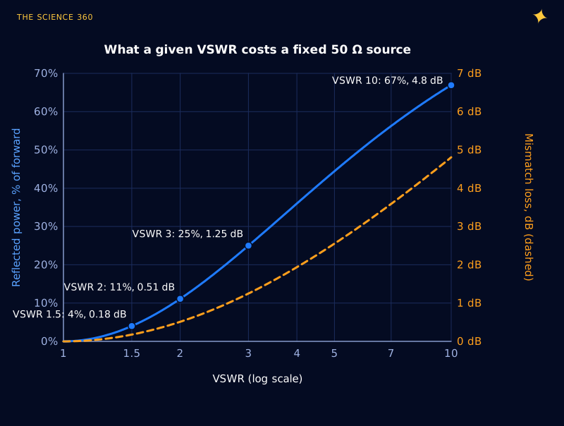
Chart of VSWR on a log axis from 1 to 10. A blue curve shows reflected power rising from 0% to 67%, with points marked at VSWR 1.5 (4%, 0.18 dB), 2 (11%, 0.51 dB), 3 (25%, 1.25 dB) and 10 (67%, 4.8 dB). A dashed orange curve on a right axis shows mismatch loss rising to 4.8 dB. — Figure 2. Reflected power and mismatch loss against VSWR. The curve is shallow near 1:1: going from 1.5 to 1.2 buys back only 0.14 dB. Above 3:1 it steepens quickly.

The low end is extremely forgiving. Going from 2 to 1.5 recovers a third of a decibel, which nobody at the other end of a link will notice; chasing 1.1:1 on an HF antenna is a hobby, not a requirement. The top end is compressed in a way that hides trouble: VSWR 10 is "only" 4.8 dB of mismatch loss, yet two thirds of the incident power is coming back.

Is reflected power lost? The misconception

The table gives 1.25 dB of mismatch loss at VSWR 3. Go back to the opening example: same antenna, VSWR 3, yet the antenna received the full 100 W. Both are correct, because they describe different systems.

The mismatch loss column assumes the generator is a fixed 50 Ω source with nothing between it and the line that can adjust. Lab signal generators often behave like this. The reflected wave returns, finds a 50 Ω source impedance that matches the line, and is absorbed there. That power really is gone, as heat inside the generator's output stage or its attenuator.

A transmitter with an antenna tuner is a different animal. The tuner is adjusted until the radio sees 50 Ω, and in doing so it presents the line with whatever impedance re-reflects the returning wave back toward the antenna, in the right phase to add to the new forward wave. Energy conservation then does the bookkeeping:

Lossless line, tuner adjusted, radio supplies 100 W net.

At the antenna:

\begin{aligned}\text{delivered} &= P_{\mathrm{fwd}} \times (1 - |\Gamma|^2) \\ &= P_{\mathrm{fwd}} \times 0.75\end{aligned}

Net into the line:

\begin{aligned}P_{\mathrm{fwd}} - P_{\mathrm{refl}} &= P_{\mathrm{fwd}} \times (1 - 0.25) \\ &= 100\ \mathrm{W} \\ P_{\mathrm{fwd}} &= 100/0.75 = \mathbf{133.3\ W} \\ P_{\mathrm{refl}} &= 0.25 \times 133.3 = \mathbf{33.3\ W}\end{aligned}

Delivered to antenna:

133.3 - 33.3 = \mathbf{100\ W}

The forward reading is higher than the radio's output because the re-reflected power is added to it. A directional wattmeter is reporting the two travelling waves on the line, not power that the radio is making and then losing. Subtract and you get the net figure, which is what the antenna gets.

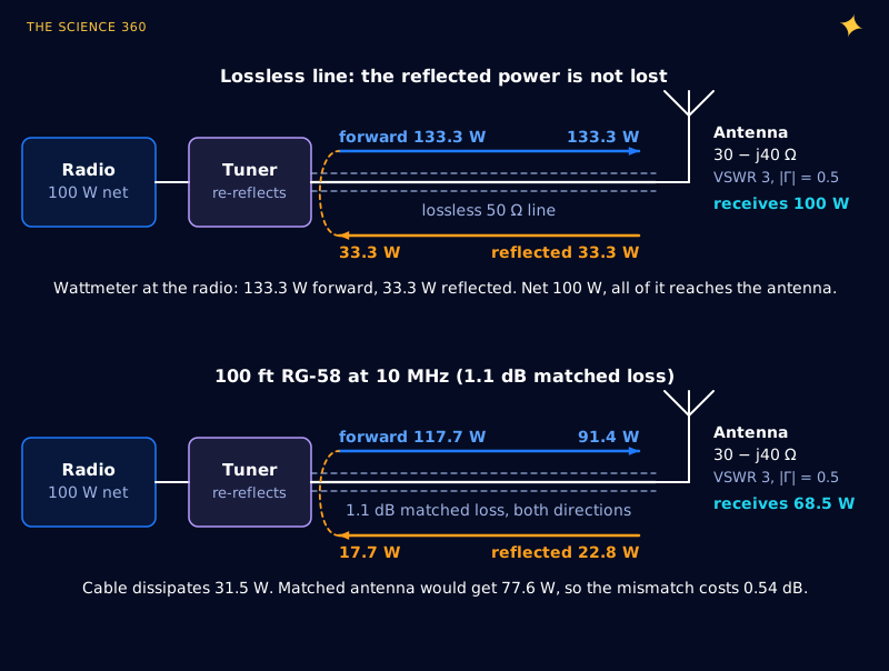
Two power flow diagrams with a radio, tuner, coax and an antenna of 30 minus j40 ohms. Top, lossless line: forward 133.3 W, reflected 33.3 W, antenna receives 100 W. Bottom, 100 feet of RG-58 at 10 MHz with 1.1 dB matched loss: forward 117.7 W at the radio and 91.4 W at the antenna, reflected 22.8 W at the antenna and 17.7 W back at the radio, antenna receives 68.5 W; the cable dissipates 31.5 W. — Figure 3. Power bookkeeping with a tuner at the radio end (our calculation). On a lossless line the reflected wave circulates and nothing is lost. On a real cable the circulating power pays the cable's attenuation on every trip.

This is the argument Walter Maxwell (W2DU) made in QST and his book Reflections, and the energy-conservation part is not controversial. Some of his further claims are: Steve Stearns (K6OIK) showed in a 2011 ARRL seminar paper that a conjugate match at only one end of a lossy line does not deliver maximum power to the load. That debate concerns fractions of a decibel. Reflected power is not automatically lost.

What a mismatch really costs: feedline loss

Real coax has loss, and that is where a high VSWR genuinely hurts. Every watt of reflected power travels the cable twice more (back, then forward again after re-reflection) and pays the attenuation each time. The larger currents and voltages of the standing wave also raise the ohmic loss in the conductors.

The standard result, published as a graph in the ARRL Antenna Book since 1949, follows directly from the bookkeeping. Let the cable's matched loss be ML dB and $a = 10^{\mathrm{ML}/10}$ . The forward wave arrives at the load reduced by a; the reflection comes back reduced by a again. The ratio of power into the line to power delivered is then:

\text{total loss} = 10\log_{10}\left[\frac{a^2 - |\Gamma_L|^2}{a\,(1 - |\Gamma_L|^2)}\right]\ \mathrm{dB}

Additional loss due to SWR:

\text{total loss} - \mathrm{ML}

Worked example: 100 ft of RG-58 at 10 MHz, antenna at VSWR 3. Belden's 8240 datasheet gives a nominal 1.1 dB per 100 ft at 10 MHz.

\begin{aligned}\mathrm{ML} &= 1.1\ \mathrm{dB} \\ a &= 10^{0.11} = 1.288 \\ a^2 &= 1.660 \\ |\Gamma_L|^2 &= 0.25 \\ \text{total loss} &= 10\log_{10}\left[\frac{1.660 - 0.25}{1.288 \times 0.75}\right] \\ &= 10\log_{10}(1.459) = \mathbf{1.64\ dB} \\ \text{additional} &= 1.64 - 1.10 = \mathbf{0.54\ dB}\end{aligned}

With 100 W into the line:

\begin{aligned}\text{delivered} &= 100/1.459 = \mathbf{68.5\ W} \\ \text{matched antenna} &= 100/1.288 \\ &= 77.6\ \mathrm{W} \\ \text{cable dissipation} &= 100 - 68.5 \\ &= \mathbf{31.5\ W}\end{aligned}

against 22.4 W if matched.

So the mismatch costs 0.54 dB here, less than the 1.25 dB "mismatch loss" in the table, because the tuner recovers the reflected power apart from what the cable eats. At 400 MHz (8.4 dB per 100 ft) a 50 ft run has 4.2 dB of matched loss, and the same antenna adds 1.09 dB on top. On a low-loss line VSWR barely matters; on a lossy line it multiplies the loss you already had.

Two panels. Left: VSWR seen at the transmitter versus VSWR at the antenna, both log scale from 1 to 10, for matched cable losses of 0, 1, 3 and 6 dB. With 3 dB of loss, VSWR 10 at the antenna appears as about 2.4 at the transmitter; with 6 dB it appears as about 1.5. Right: additional loss in dB versus VSWR at the antenna for matched losses of 0.5, 1, 2 and 4 dB, rising to between 1.5 and 4.3 dB at VSWR 10. — Figure 4. Left: cable loss hides the mismatch from the radio, since $|\Gamma_{\mathrm{TX}}| = |\Gamma_L|/a$ . Right: additional loss from the formula above. Both computed by us from the standard lossy-line relations.

Why a low SWR reading can be bad news

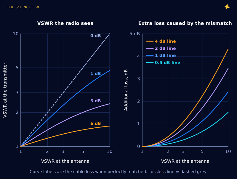
The left panel of Figure 4 is the trap. The reflected wave is attenuated on its way back, so the radio sees a smaller mismatch than the antenna has. With 3 dB of cable loss, an antenna at 10:1 reads about 2.4:1 at the radio; with 6 dB of loss it reads about 1.5:1. Take the 400 MHz example again:

50 ft RG-58 at 400 MHz:

\begin{aligned}\mathrm{ML} &= 4.2\ \mathrm{dB} \to a = 2.630 \\ |\Gamma_{\mathrm{TX}}| &= |\Gamma_L|/a = 0.5/2.630 \\ &= 0.190\end{aligned}

VSWR at the radio:

\frac{1 + 0.190}{1 - 0.190} = \mathbf{1.47}

though the antenna is at 3.0.

A long run of thin cable is an attenuator, and an attenuator looks like a good match from its input whatever sits on the far end. If a VHF or UHF system shows an excellent SWR that does not change when you detune the antenna, suspect the cable or a waterlogged connector. Measure at the antenna end, or measure the cable loss on its own.

Does reflected power heat the transmitter?

Here the conclusion (a bad mismatch can kill a transmitter) is right and the usual mechanism is wrong. The popular picture is the reflected wave running back into the output stage and being absorbed like heat in a resistor. That needs the output stage to look like a 50 Ω resistor, and a power amplifier does not. Ampleon's BLF188XR, a 1.4 kW LDMOS transistor for HF to 600 MHz, wants a load of $2.74 + j0.57\ \Omega$ at 108 MHz according to its datasheet, at 73% drain efficiency. The output network transforms the 50 Ω connector down to those few ohms.

What the reflected wave actually does is change the load impedance the transistor sees. Transformed back through the line and output network, a VSWR 3 antenna shows up at the drain as some impedance on a VSWR 3 circle around the intended 2.74 Ω, at an angle set by the cable length. Depending on where it lands:

A higher impedance raises the RF voltage swing at the drain toward its breakdown limit, while the current falls.
A lower impedance raises the current and the $I^2R$ loss in the device, while the voltage falls.
A reactive impedance costs efficiency, so dissipation (DC in minus RF out) rises.

The reflected power is the same 25% at every phase of a VSWR 3 load, yet the stress on the transistor is not, so the reflected watts are not what does the damage. That is why ruggedness is specified "through all phases": the BLF188XR withstands VSWR greater than 65:1 through all phases at 1,400 W pulsed. Consumer radios are rarely that tough, so they measure VSWR and fold back their power instead.

There is one common case where the reflected power really is dumped as heat: transmitters with a circulator or isolator on the output. The circulator steers the returning wave into a 50 Ω load resistor built to absorb it. A magnetron in an empty microwave oven faces a large mismatch too (see why metal sparks in a microwave for what the high field in an unloaded cavity does).

Source note The statements that "most solid-state radios" begin cutting power somewhere around 2:1 to 3:1 come from general experience and the electronics-notes overview, not from a specific manufacturer's manual. Thresholds vary between models; check the manual for your own radio.

Voltage and current peaks along a mismatched line

The other real cost is local: some points on the line carry more voltage, and others more current, than in the matched case. For the $30 - j40\ \Omega$ antenna with 100 W delivered:

\begin{aligned}P_{\mathrm{fwd}} &= 133.3\ \mathrm{W} \\ V_{\mathrm{fwd}} &= \sqrt{133.3 \times 50} = 81.6\ \mathrm{V\ rms} \\ I_{\mathrm{fwd}} &= 81.6/50 = 1.63\ \mathrm{A\ rms} \\ V_{\max} &= 81.6 \times 1.5 = \mathbf{122.5\ V\ rms} \\ &\ \ (173\ \mathrm{V\ peak}) \\ V_{\min} &= 81.6 \times 0.5 = \mathbf{40.8\ V\ rms} \\ I_{\max} &= 1.63 \times 1.5 = \mathbf{2.45\ A\ rms} \\ I_{\min} &= 0.82\ \mathrm{A\ rms}\end{aligned}

Matched line at 100 W: 70.7 V rms and 1.41 A rms everywhere.

$I^2R$ heating at a current peak relative to matched:

(2.45/1.41)^2 = \mathbf{3.0\ times}

RMS voltage and current along a lossless 50 ohm line feeding a 30 minus j40 ohm antenna with 100 watts delivered, over 0.75 wavelength. Voltage, solid blue, swings between 40.8 and 122.5 volts. Current, dashed orange, swings between 0.82 and 2.45 amps. The voltage peaks sit where the current dips, a quarter wavelength apart. — Figure 5. Voltage and current along the line for the worked example (our calculation). Because the load is capacitive, a voltage minimum appears first, 0.125 λ back from the antenna. The product $V_{\min} \times I_{\max} = 40.8 \times 2.45 = 100\ \mathrm{W}$ .

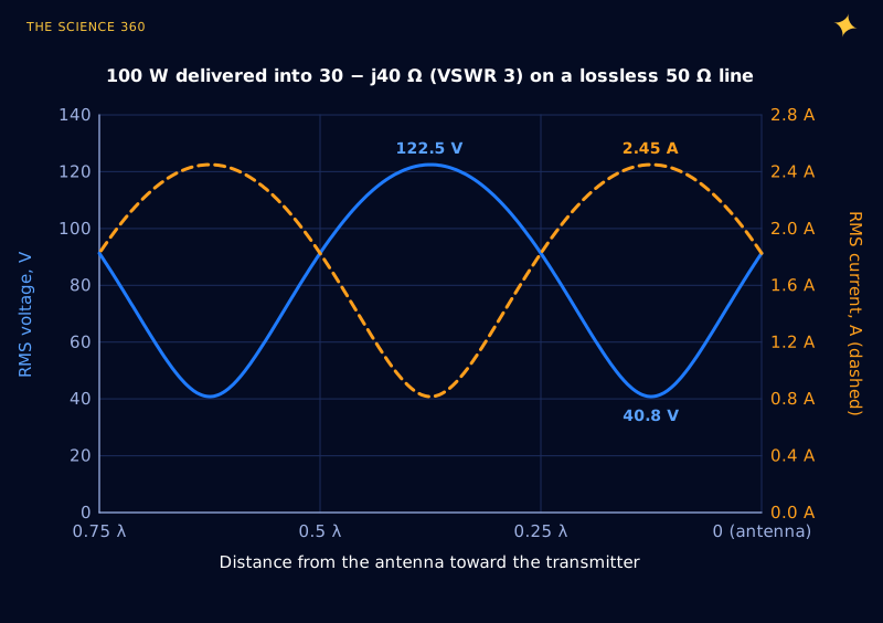
At 100 W that is harmless. At 1.5 kW into VSWR 10, the forward power is $1{,}500/(1 - 0.818^2) = 4{,}540\ \mathrm{W}$ and the voltage peaks reach $476 \times 1.818 = 866\ \mathrm{V\ rms}$ , about 1,225 V peak. The current peaks heat the cable at fixed spots, and at RF that current is crowded into a thin surface layer (see skin effect and skin depth), which is why cable loss climbs with frequency in the first place.

How to bring VSWR down, and when not to bother

If the antenna's feedpoint impedance is wrong, adjust the antenna: length first (a quarter-wave antenna a few percent short is capacitive, like our $30 - j40\ \Omega$ example), then the ground plane. Otherwise, a matching network at the antenna end fixes the VSWR on the whole feedline and removes the extra cable loss; a tuner at the radio end only keeps the radio happy. Matching networks are LC circuits, so they are narrowband by nature.

A practical scale, using the numbers above: below 1.5:1, stop. Between 1.5 and 2, fine for nearly all receive and most transmit work, with mismatch loss under 0.51 dB. Between 2 and 3, acceptable on a short low-loss line with a tuner; check that the radio is not folding back. Above 3, fix it, especially at VHF and up where cable loss is high and the additional-loss curves in Figure 4 climb fast.

The short version for your bench:

|\Gamma| = (\text{VSWR} - 1)/(\text{VSWR} + 1)

;

\text{return loss} = -20\log|\Gamma|

;

\text{reflected power} = |\Gamma|^2

. VSWR 2 means 11% reflected and 9.5 dB return loss. Reflected power is only lost outright into a fixed 50 Ω source; with a tuner it circulates and the real cost is extra cable loss. A transmitter suffers because a mismatch changes its load impedance, not because it absorbs the reflected watts. And a perfect SWR at the end of a long, thin cable is a warning, not a reassurance.

FAQ

What is a good VSWR?

Below 1.5:1 is good for almost anything, since it reflects only 4% of the forward power. 2:1 (11% reflected, 0.51 dB of mismatch loss into a fixed 50 Ω source) is the usual acceptance limit for antennas and radios. Above 3:1 most solid-state transmitters reduce their output to protect themselves, and feedline loss starts to rise noticeably.

How do you convert VSWR to return loss?

First find the reflection coefficient magnitude, $|\Gamma| = (\text{VSWR} - 1)/(\text{VSWR} + 1)$ . Return loss in dB is then $-20\log_{10}|\Gamma|$ . VSWR 2 gives $|\Gamma| = 0.333$ and a return loss of 9.54 dB; VSWR 1.5 gives 0.2 and 13.98 dB. Return loss is a positive number for any passive load.

Does high VSWR damage a transmitter?

It can, but not because reflected power flows back and is burned up like heat in a resistor. A mismatch changes the impedance the output transistors see, which can raise their peak voltage, their peak current or their dissipation depending on the phase of the reflection. Most modern radios measure VSWR and cut their power before that happens.

Where does reflected power go?

It travels back down the feedline to the transmitter end. If a tuner or matching network there presents the right impedance, it is re-reflected toward the antenna, and on a lossless line all of it is eventually delivered. The real cost is that the extra circulating power passes through a lossy cable more than once, so the cable dissipates more.

Why does my SWR look better at the radio than at the antenna?

Feedline loss attenuates the reflected wave on its way back, so the radio sees a smaller reflection than the antenna produces. 3 dB of matched cable loss turns a 10:1 VSWR at the antenna into about 2.4:1 at the radio. A suspiciously perfect SWR on a long or thin cable often means the cable is eating the power.

Sources

Keysight, VSWR and return loss calculator ( $\text{return loss} = -20\log|\Gamma|$ , $\text{VSWR} = (1 + |\Gamma|)/(1 - |\Gamma|)$ ): keysight.com VSWR return loss calculator
Electronics Notes, "What is VSWR" (typical page-one explanation; foldback, feeder heating): electronics-notes.com what-is-vswr
Trevor S. Bird, "Definition and Misuse of Return Loss," IEEE Antennas and Propagation Magazine 51(2), 166 to 167, 2009, doi:10.1109/MAP.2009.5162049: researchers.mq.edu.au record
Steve Stearns, K6OIK, "Conjugate Match Myths," ARRL Pacificon Antenna Seminar, 2011 (lossy-line power flow, ARRL additional-loss formula, critique of Maxwell): fars.k6ya.org Stearns PDF
Belden 8240 RG-58/U coax technical data (1.1 dB/100 ft at 10 MHz, 8.4 dB/100 ft at 400 MHz): Belden 8240 datasheet (TME copy)
Ampleon BLF188XR / BLF188XRS power LDMOS transistor datasheet (VSWR > 65:1 ruggedness, $Z_L = 2.74 + j0.57\ \Omega$ , 73% efficiency): BLF188XR datasheet PDF

Method note: all curves are computed from the lossless and lossy transmission-line relations given in the text (Python, numpy). Figure 3 and the worked examples assume an ideal tuner at the radio end that presents the radio with 50 Ω. Cable loss is treated as the same in both directions and independent of the standing wave, the same approximation used in the ARRL additional-loss chart.

Header image: NASA/JPL-Caltech (image PIA24163), regraded for this article.