How much does sunlight change around a planetary orbit? A Python comparison

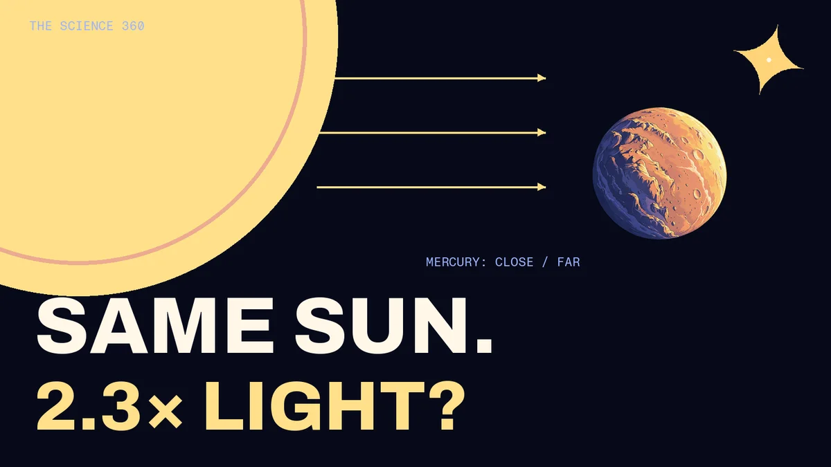
A planet does not receive the same intensity of sunlight throughout an elliptical orbit. Using one fixed set of JPL orbital elements, we calculate a close-to-far increase of 6.9% for the Earth–Moon system, 45.5% for Mars and 130.4% for Mercury. Those percentages compare each body’s closest point with its own farthest point. They do not compare the planets’ climates.

The surprisingly useful result is that this particular ratio depends on the orbit’s eccentricity, not its overall size. We can therefore compare orbital shape without confusing it with the much larger difference between being near the Sun and living far away.

Below is a reproducible calculation from published parameters, rather than new observations or a forecast for a particular date. It also explains why the result does not overturn the familiar explanation of Earth’s seasons.

The question we can actually calculate

Imagine an identical detector facing directly toward the Sun, above each planet’s atmosphere. Compare the light power reaching a square metre at the closest and farthest parts of that planet’s orbit. Keep the Sun’s output constant. Ignore clouds, rotation, dust, tilt and the detector’s temperature.

This intentionally restricted question concerns irradiance normal to the incoming rays. It does not describe the energy reaching a patch of ground over a day. NASA’s inverse-square lesson supplies the underlying relationship: illumination falls as distance squared increases. Applying that relationship to an ellipse gives us a clean calculation.

For an ellipse with semimajor axis a and eccentricity e:

closest distance = a × (1 − e)
farthest distance = a × (1 + e)
close / far irradiance = ((1 + e) / (1 − e))²
increase from farthest = 100 × (ratio − 1) percent

The factor a cancels in the ratio. It remains essential if we want absolute irradiance or want to compare one planet’s light level with another’s.

One parameter table, eight comparisons

We use the J2000 base values in JPL’s approximate planetary-elements table for the 1800–2050 fit. We freeze those base values instead of advancing them to 2026. JPL’s Earth entry is the Earth–Moon barycenter, the system’s shared centre of mass; the table below preserves that distinction.

These are representative fixed orbital shapes, not precise perihelion and aphelion predictions for this year. JPL documents approximation errors for its position method; the extra digits in our CSV do not remove those limitations.

Body	Eccentricity used	Close / far irradiance	Increase from farthest
Mercury	0.20563593	2.304×	130.4%
Venus	0.00677672	1.027×	2.7%
Earth–Moon barycenter	0.01671123	1.069×	6.9%
Mars	0.09339410	1.455×	45.5%
Jupiter	0.04838624	1.214×	21.4%
Saturn	0.05386179	1.241×	24.1%
Uranus	0.04725744	1.208×	20.8%
Neptune	0.00859048	1.035×	3.5%

The result makes two useful comparisons visible. Mercury’s large fractional swing is unsurprising once its eccentricity is included. Neptune, despite being far from the Sun, has a smaller fractional swing than Earth because its orbit in this parameter set is closer to circular. Distance determines the underlying light level; eccentricity determines this particular relative swing.

A denominator can change the headline

For Mars, the close-point irradiance is about 45.5% greater than the far-point irradiance. Reversing the comparison does not give a 45.5% decrease. The far-point level is about 31.2% lower than the close-point level, because that percentage uses the larger number as its denominator.

The two descriptions are consistent: divide the same difference by a different reference level and you get a different percentage. When comparing claims about planetary sunlight, first check whether the author means close versus far, far versus close, or deviation from a reference distance.

Our downloaded results also include light levels relative to each body’s own semimajor-axis distance. For the Earth–Moon entry, the endpoints are roughly 1.034 and 0.967 in those units. The endpoint ratio is 1.069. Adding rounded positive and negative deviations is only an approximation to that ratio.

Why this does not explain Earth’s summer

Distance affects incoming light, but Earth’s opposite hemispheric seasons primarily follow its axial tilt. The Northern Hemisphere experiences winter around Earth’s closest approach to the Sun and summer around its farthest. NASA Space Place’s explanation distinguishes the seasonal tilt effect from the smaller Earth–Sun distance variation.

Our detector experiment intentionally removed the factors that produce local seasons: the angle at which rays strike a surface and the time that surface spends in daylight. A calculation that excludes those factors cannot predict a city’s summer temperature.

The same caution becomes even more useful on Mars. NASA’s Mars overview describes an elliptical orbit, axial tilt and an atmosphere that all matter for its environment. Our 45.5% result isolates one geometric effect. It is not a prediction that a thermometer will rise by 45.5%, nor that a solar panel will produce 45.5% more electricity.

Reproduce the calculation

Download the parameter CSV, complete Python script, result CSV and provenance notes. Save the script and input CSV in one folder, then run python analyze.py. It uses only Python’s standard library.

The essential calculation is short:

import csv

with open('orbital-elements.csv', encoding='utf-8') as stream:
    for row in csv.DictReader(stream):
        e = float(row['eccentricity'])
        ratio = ((1 + e) / (1 - e)) ** 2
        print(row['body'], round(100 * (ratio - 1), 1))

The full script independently calculates the closest and farthest distances, checks that their squared ratio agrees with the simplified expression, and verifies that a circular orbit gives a ratio of one. These checks catch formula and parsing mistakes; they do not turn an approximate orbital model into an exact ephemeris.

There are no statistical confidence bands here. We have evaluated a deterministic formula using a published approximate parameter set, without propagating orbital-fit uncertainty. Solar-output variability, planetary perturbations over time and surface processes are outside the model. Use a dated ephemeris and a fuller illumination model for engineering or observing work that needs those details.

For another way orbital geometry shapes what we see, read our explanation of retrograde motion. The useful habit is the same: identify the geometry being calculated before attaching a larger physical story to the number.

Cover: conceptual AI-assisted planetary artwork with an independently composed Sun, typography and vector star. It is not a telescope image, geographic map or scale drawing. The article chart is generated from the linked calculation.