Electric Field Lines: Rules and Diagrams for Every Case • The Science 360

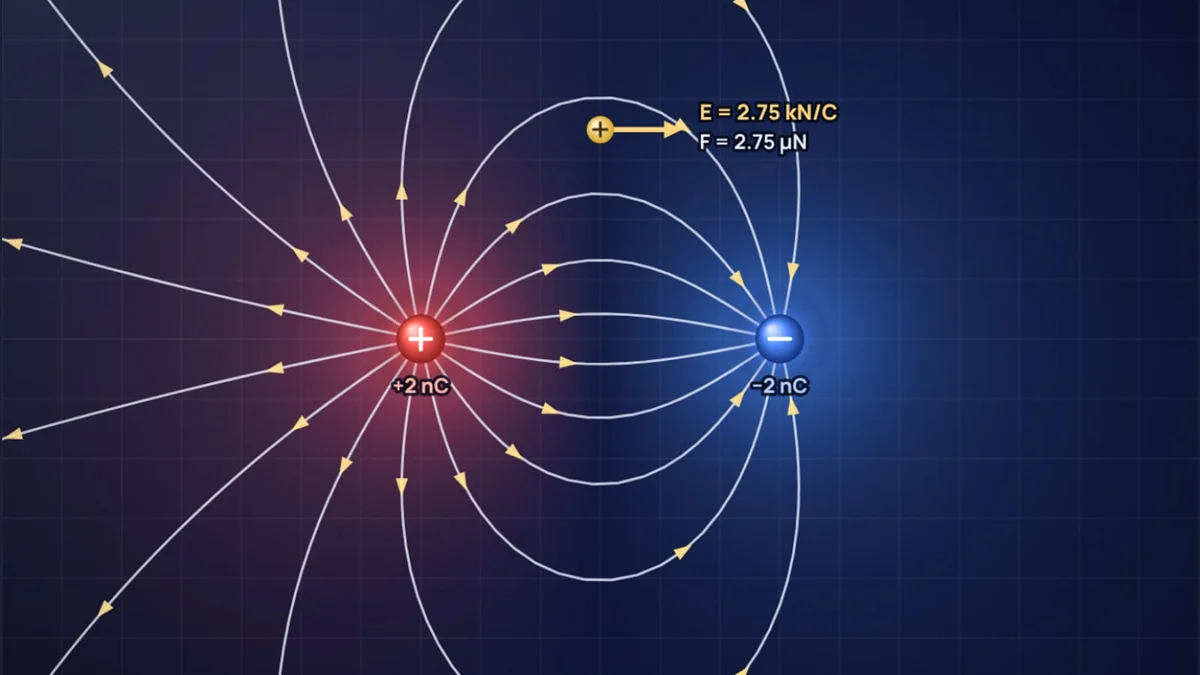
An electric field is invisible, so physicists draw it. A field line is a curve whose direction at every point is the direction a small positive charge would be pushed. Draw enough of them by a few simple rules and the picture tells you the direction of the force everywhere, roughly how strong it is, and where it vanishes. This guide goes through those rules and then applies them to every arrangement that comes up in Class 12 and first year physics. Every diagram here was drawn by our electric field lines simulator, which traces the lines from Coulomb's law and lets you drag the charges around.

Quick answerElectric field lines start on positive charges and end on negative charges (or at infinity). The number of lines is proportional to the charge. The field at any point is tangent to the line through it. Lines crowd where the field is strong and spread where it is weak. Two lines never cross, and every line meets an equipotential surface at a right angle.

The five rules of electric field lines

OpenStax College Physics lists the properties of field lines as five rules. Everything else in this guide follows from them.

Rule	What it means on a diagram	Why it holds
Lines begin on positive charges and end on negative charges	Arrows point away from + and into −; unmatched lines go to infinity	The field points the way a positive test charge would be pushed
The number of lines is proportional to the charge	A +3 nC charge gets three times as many lines as a +1 nC charge	Gauss's law: the flux out of a charge is q/ε₀
Line density shows field strength	Crowded lines mean a strong field, sparse lines a weak one	The same lines spread over a larger area farther out
The field is tangent to the line	Draw the tangent at a point to find the force direction there	That is how a field line is defined
Lines never cross	Two lines can only meet at a null point, where E = 0	The field has one direction at each point

A sixth rule comes in once you add potential: field lines cross equipotential surfaces at right angles. We come back to that at the end.

The simulator follows the second rule literally. It gives each charge 8 lines per nanocoulomb, so a 2 nC charge sends out 16 lines and a 3 nC charge sends out 24. It then traces each line step by step, always moving along the local field, until the line reaches a negative charge or leaves the screen.

A single point charge

Start with one positive charge on its own. The lines go straight out in every direction, evenly spaced, like spokes. For a negative charge the picture is the same with the arrows reversed. The field strength comes from Coulomb's law:

\begin{aligned}E &= \frac{1}{4\pi\varepsilon_0}\,\frac{q}{r^2} = k\,\frac{q}{r^2} \\ k &= 8.988 \times 10^{9}\ \mathrm{N\,m^2\,C^{-2}}\end{aligned}

The value of k comes from the vacuum permittivity, $\varepsilon_0 = 8.854 \times 10^{-12}\ \mathrm{F/m}$ , as listed by NIST.

Worked example: the field of a 2 nC charge

\begin{aligned}E(10\ \mathrm{cm}) &= \frac{8.988\times10^{9} \times 2\times10^{-9}}{(0.10)^2} \\ &= 1.80\times10^{3}\ \mathrm{N/C} \\ E(5\ \mathrm{cm}) &= \frac{17.98}{(0.05)^2} \\ &= 7.19\times10^{3}\ \mathrm{N/C} \\ V(10\ \mathrm{cm}) &= \frac{kq}{r} = \frac{17.98}{0.10} = 180\ \mathrm{V}\end{aligned}

Halving the distance makes the field four times stronger. On the diagram the same 16 lines are packed onto a circle half as big, so they are twice as close in each direction.

This is why line density works as a measure of strength. In three dimensions the lines spread over a sphere of area $4\pi r^2$ , so their density falls as $1/r^2$ , exactly like Coulomb's law. On a flat drawing the spacing only falls as 1/r, so a 2D diagram gives you a fair sense of where the field is strong but not an exact ratio. Treat line pictures as qualitative and use the numbers for anything quantitative.

Electric dipole: a positive and a negative charge

Put +2 nC and −2 nC charges 12 cm apart and you get the most familiar field diagram in physics. Lines leave the positive charge, bend round and enter the negative one. Because the two charges are equal, every one of the 16 lines that leaves the positive charge ends on the negative charge. None escape to infinity, which you can only see if you look far enough out: the outermost lines take very wide loops.

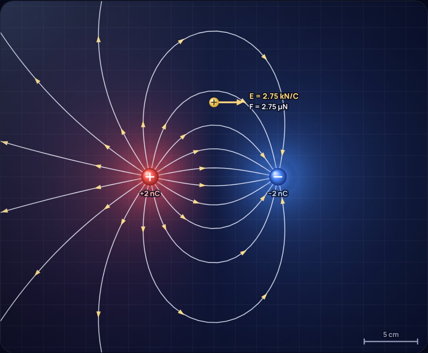
Electric field lines of a dipole: lines leave a +2 nC charge and curve into a -2 nC charge 12 cm away, with arrows, red and blue potential shading and a test charge feeling a 2.75 kN/C field — Figure 1. A dipole, +2 nC and −2 nC 12 cm apart. The lines are densest on the axis between the charges, where the field is strongest. The red shading marks positive potential and the blue negative. Open this setup in the simulator.

Between the charges the two fields point the same way, from + towards −, so they add. At the midpoint each charge is 6 cm away:

Worked example: the dipole at its midpoint and above it

\begin{aligned}E_{\text{mid}} &= 2 \times \frac{kq}{r^2} = 2 \times \frac{17.98}{(0.06)^2} \\ &= 9.99\times10^{3}\ \mathrm{N/C} \\ V_{\text{mid}} &= \frac{kq}{r} + \frac{k(-q)}{r} = 0\end{aligned}

Now move 7 cm straight up from the midpoint. Each charge is $\sqrt{6^2 + 7^2} = 9.22$ cm away and contributes $17.98/(0.0922)^2 = 2.11$ kN/C. The vertical parts cancel and the horizontal parts, each a fraction 6/9.22 of that, add:

E = 2 \times 2.11 \times \frac{6}{9.22} = 2.75\times10^{3}\ \mathrm{N/C}

A 1 nC test charge there feels $F = qE = 10^{-9} \times 2750 = 2.75\ \mu\mathrm{N}$ , pointing parallel to the axis, from the + side towards the − side.

The midpoint result is worth remembering. The field there is strong, almost 10 kN/C, yet the potential is zero. Field and potential are different things: the field is about the slope of the potential, not its value.

Two like charges and the null point

Now make both charges +2 nC. The lines from each charge bend away from the other one, and none of them join the two charges. Between the charges there is a gap with no lines at all, and in the middle of it the field is exactly zero.

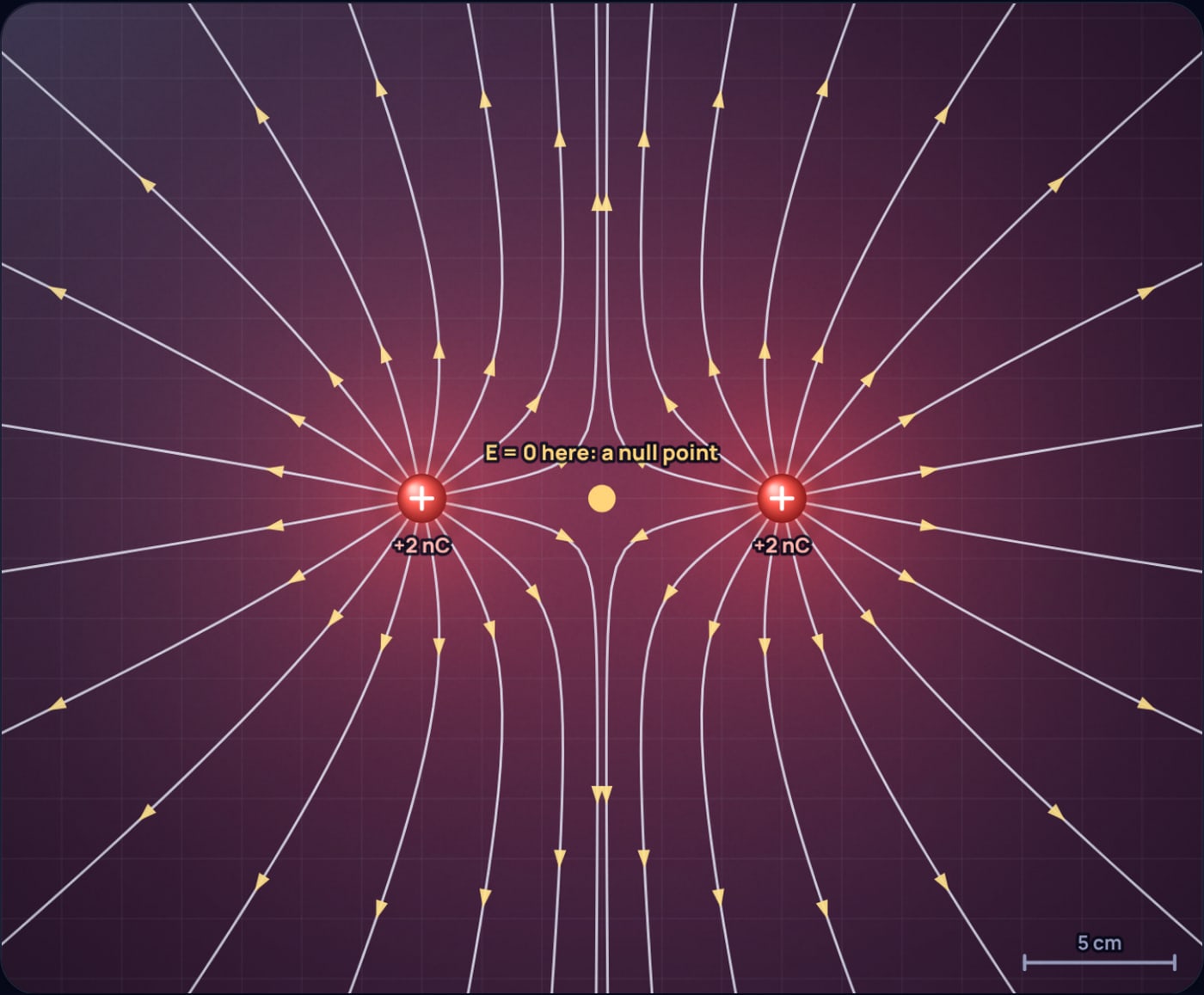
Electric field lines of two equal positive charges, +2 nC each, 12 cm apart: the lines push away from each other and leave a null point midway where the field is zero — Figure 2. Two +2 nC charges 12 cm apart. The lines repel each other and all 32 run off to infinity. The test charge sits on the null point, where the two fields cancel. Open this setup in the simulator.

At the midpoint the two charges push a test charge with equal and opposite forces, so the net field is zero. This is the null point, and it is the only place two field lines can meet: with no field there is no direction, so the rule against crossing does not apply. The potential is not zero, though. Each charge contributes 300 V, so $V = 2 \times 17.98/0.06 = 599$ V. Move 7 cm up from the midpoint and the field rises to 3.21 kN/C, pointing straight up, away from both charges.

The repulsion you see in the diagram is real. The force between the two charges is

\begin{aligned}F &= \frac{k q_1 q_2}{r^2} \\ &= \frac{8.988\times10^{9} \times (2\times10^{-9})^2}{(0.12)^2} \\ &= 2.50\ \mu\mathrm{N}\end{aligned}

Faraday described field lines as if they were stretched rubber bands that also push sideways on each other. That picture is useful here: the lines between like charges push apart, which is a way of seeing why the charges repel.

Unequal charges: +3 nC and −1 nC

Unequal charges are where the line counting rule earns its place. A +3 nC charge sends out 24 lines, and a −1 nC charge only takes in 8. So 8 lines run from the big charge to the small one, and the other 16 have nowhere to end and head out to infinity. Far away, the pair looks like a single +2 nC charge, because that is the net charge.

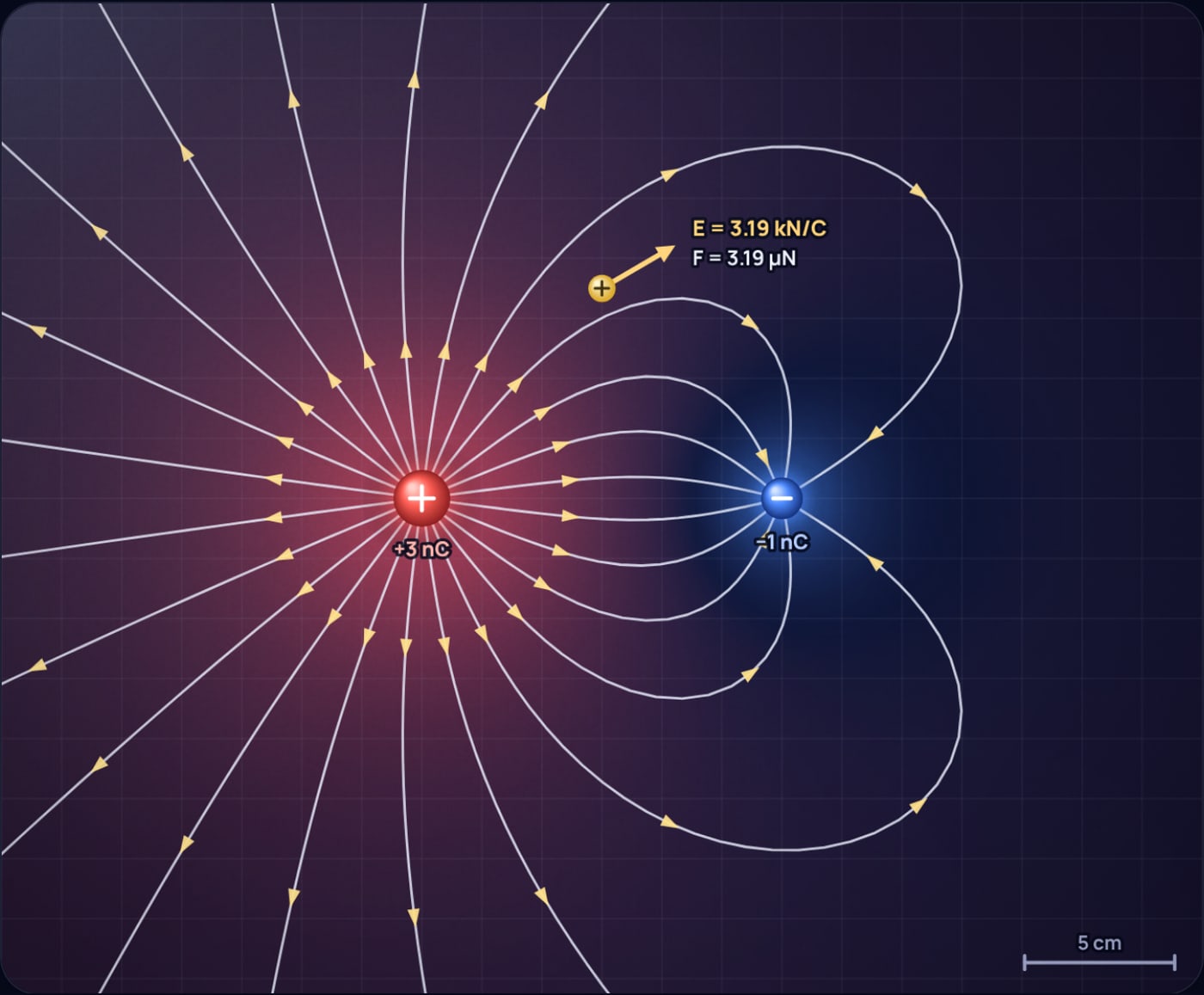
Electric field lines of a +3 nC and a -1 nC charge: 8 of the 24 lines from the larger charge end on the smaller one and the rest run off to infinity — Figure 3. +3 nC and −1 nC, 12 cm apart. Only a third of the lines from the positive charge end on the negative one. Open this setup in the simulator.

There is still a null point, but it is not between the charges. Between them both fields point towards the negative charge, so they cannot cancel. It sits outside, on the far side of the smaller charge, where the weak nearby charge balances the strong distant one. With the +3 nC charge at x = −6 cm and the −1 nC charge at x = +6 cm, call d the distance beyond the small charge:

\begin{aligned}\frac{3}{(d + 12)^2} &= \frac{1}{d^2} \\ d + 12 &= \sqrt{3}\,d \\ d &= \frac{12}{\sqrt{3}-1} = 16.4\ \mathrm{cm}\end{aligned}

So the null point is at x = 22.4 cm. In the simulator you can drag the test charge along the axis and watch the field fall to zero there and then reverse. The general rule: for opposite charges, the null point is outside the pair, nearer the smaller charge. For like charges it is between them, again nearer the smaller one.

Parallel plates: a nearly uniform field

A charged plate can be modelled as many point charges in a row. The simulator uses two rows of 11 charges, each ±0.5 nC, along lines 10 cm apart and 20 cm long. Between the rows the field lines run straight across and evenly spaced. Near the ends they bulge outwards. This bulge is called the fringing field.

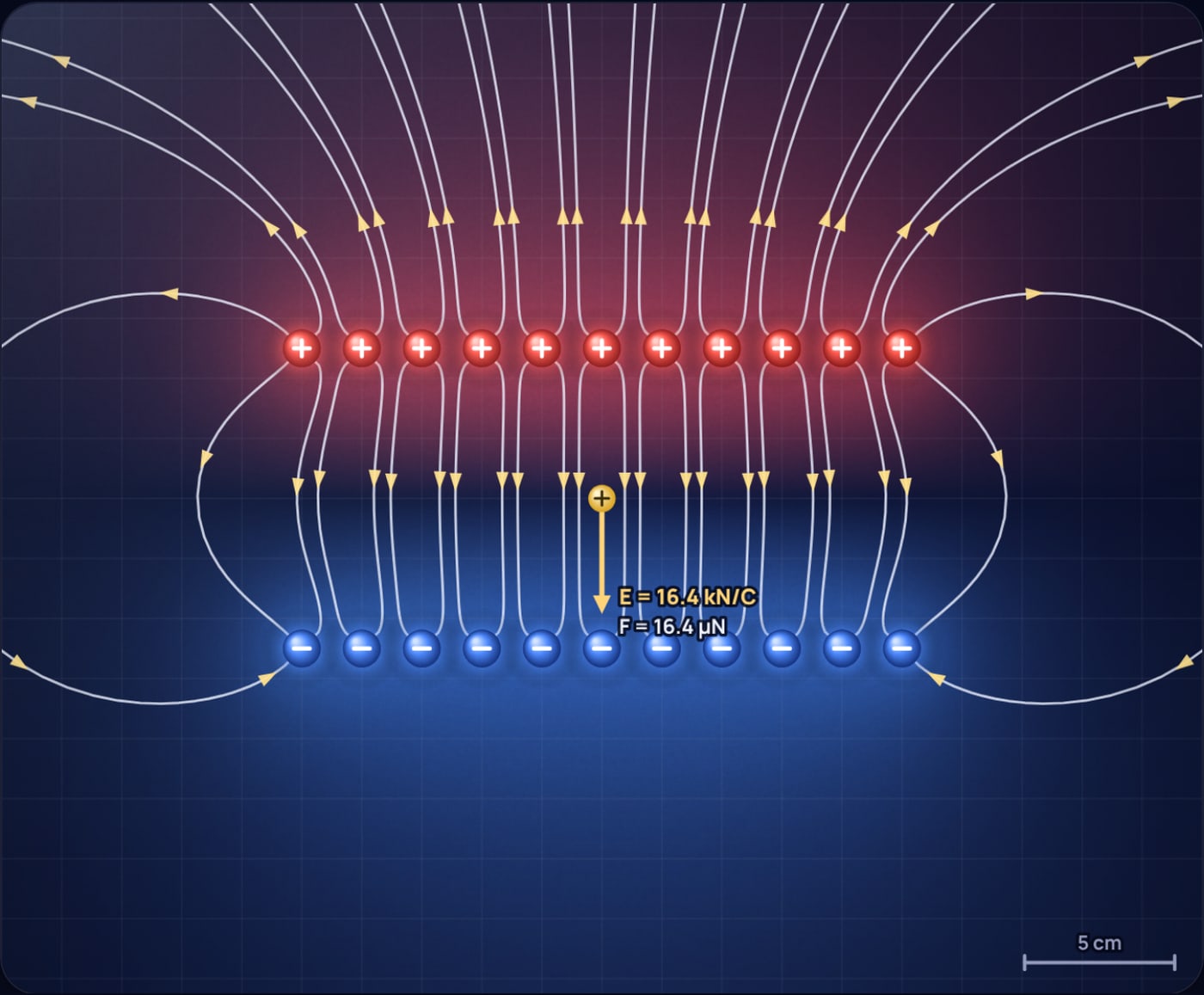
Electric field between two parallel rows of charge 10 cm apart: straight, evenly spaced field lines from the positive to the negative plate with a 16.4 kN/C field at the centre and fringing lines bulging out at the ends — Figure 4. Two rows of charge modelling parallel plates. In the middle the lines are straight and evenly spaced; at the ends they bow outwards. Open this setup in the simulator.

Straight, parallel, evenly spaced lines are the signature of a uniform field, and this is why a parallel plate capacitor is the standard way to make one. With the model in the simulator the field at the centre is 16.4 kN/C. It is 17.1 kN/C 1 cm above the centre and 19.9 kN/C 2 cm above, so it is close to uniform in the middle and grows as you approach a row of separate point charges. Real plates carry a continuous charge rather than 11 dots, and plates that are wide compared with their gap give a field that is uniform over almost the whole space between them.

Quadrupole: four charges, one null point

Place +2 nC and −2 nC charges alternately on the corners of a 12 cm square. Each positive charge sends its lines to the two negative neighbours, so the lines form four curved bundles around the edges of the square. At the centre everything cancels: the field is zero, and the potential is zero as well.

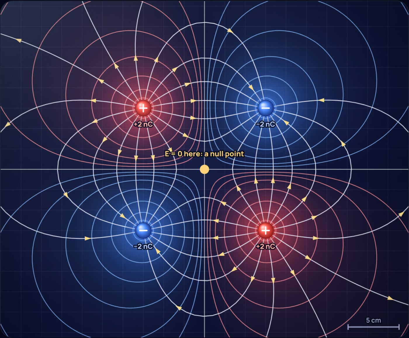
Electric field lines and dashed equipotential lines of a quadrupole, alternating +2 nC and -2 nC charges on a 12 cm square, with a null point of zero field at the centre — Figure 5. A quadrupole with equipotential lines switched on. The field is zero at the centre and rises quickly away from it. Open this setup in the simulator.

The field around the centre grows fast. At 4 cm above the centre it is already 7.17 kN/C. Because the net charge and the net dipole moment are both zero, the field far away falls off much faster than for a single charge or a dipole, which is why quadrupole lines stay close to the charges.

Equipotentials and the right angle rule

An equipotential is a line (in 3D, a surface) along which the potential is the same everywhere. Moving a charge along it takes no work, because $W = q\,\Delta V = 0$ . But work is force times displacement along the force. If no work is done for any small step along the equipotential, the field must have no component along it. So the field, and every field line, crosses each equipotential at 90°.

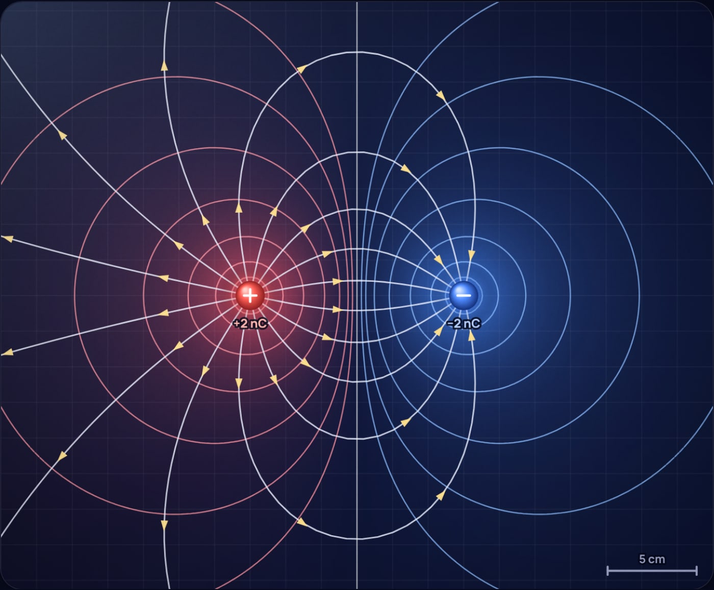
Dipole with equipotential lines: circles of equal potential around the +2 nC and -2 nC charges, the straight 0 V line midway, and field lines crossing every equipotential at right angles — Figure 6. A dipole with equipotentials. Near each charge they are almost circles. The midline is the 0 V equipotential, and every field line crosses it at a right angle. Open this setup in the simulator.

Close to a charge, the equipotentials are nearly circles, because that charge dominates. Halfway between the two charges of a dipole, the 0 V equipotential is a straight line: the perpendicular bisector. The equipotentials are also closest together where the field is strongest. That follows from $E = -\,dV/dr$ : a steep fall in potential means a strong field.

Common mistakes in field line diagrams

Drawing lines that cross. If your sketch has two lines crossing, one of them is wrong. Only at a null point do lines meet.
Same number of lines on unequal charges. A +3 nC charge needs three times the lines of a −1 nC charge, and the extra lines must leave the picture.
Lines joining like charges. Lines never run from one positive charge to another. They bend away from each other.
Treating a field line as a path. A field line shows the direction of the force, not the path a charge would follow. A charge that starts moving will curve off the line because of its own inertia.
Arrows missing. Without arrows a dipole diagram looks identical whichever charge is positive.

Try it yourself

The best way to make these rules stick is to break things and watch the lines respond. In the electric field lines simulator you can drag any charge, change its size and sign, add or remove charges, and move the test charge around to read the field, potential and force. Try pulling the two charges of a dipole far apart and watch the lines straighten, or make a pair of like charges unequal and follow the null point as it slides towards the smaller charge.

If you want to see what large fields do in the real world, read why birds sitting on a power line don't get electrocuted, what happens when a strong field pulls electrons off metal in a microwave, and how much energy a single lightning bolt really carries.

Sources

NIST, CODATA 2022 value of the vacuum electric permittivity ε₀ = 8.8541878188 × 10⁻¹² F/m: physics.nist.gov
OpenStax, College Physics 2e, section 18.5 "Electric Field Lines: Multiple Charges" (the five properties of field lines): openstax.org

Frequently asked questions

Why do electric field lines never cross?

At any point the electric field has exactly one direction, and a field line points along that direction. If two lines crossed, the field at the crossing would point two ways at once, which is impossible. The only places where lines seem to meet are null points, where the field is zero and has no direction at all.

Where do electric field lines start and end?

They start on positive charges and end on negative charges. If the charges are not balanced, the extra lines run off to infinity, or come in from infinity to end on the extra negative charge.

What does the spacing of field lines tell you?

How strong the field is. Where lines crowd together the field is strong, and where they spread apart it is weak. Around a single point charge the lines spread over a sphere, so their density falls as 1/r squared, the same way Coulomb’s law does.

Is the electric field zero between two like charges?

Only at one point. For two equal positive charges the field is zero exactly midway between them, the null point. Everywhere else on the line joining them it points away from the nearer charge. The potential at that point is not zero; for two 2 nC charges 12 cm apart it is about 599 V.

Are equipotential lines always perpendicular to field lines?

Yes. Moving along an equipotential takes no work, so the field can have no component along it. That means the field, and every field line, crosses each equipotential at a right angle.