What do electric field lines show?
Electric field lines are a map of the force a small positive charge would feel. At every point the line runs in the direction of the field, so a positive test charge would be pushed along it. Lines start on positive charges and end on negative ones, never cross, and are drawn closer together where the field is stronger. The number of lines leaving a charge is proportional to its size, so a 2 nC charge gets twice as many as a 1 nC charge.
Behind every line is Coulomb's law. A point charge q makes a field E = kq/r², with k = 8.988 × 10⁹ N m²/C². For the 2 nC charge in the simulation that is 1.80 kN/C at 10 cm and 7.19 kN/C at 5 cm: half the distance, four times the field. With several charges the fields add as vectors, and the simulation traces the lines through that sum. For a feel of what these fields do in nature, see why birds do not get electrocuted and the lightning physics of Back to the Future.
Key results from the simulation
- Inverse square: a 2 nC charge gives 1.80 kN/C at 10 cm and 7.19 kN/C at 5 cm, and a potential of 180 V at 10 cm.
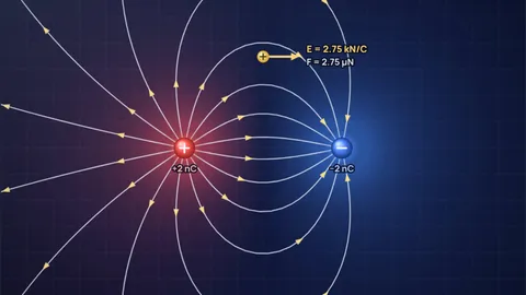
- Dipole: with +2 nC and −2 nC 12 cm apart, the field midway is 9.99 kN/C, pointing from + to −, while the potential there is exactly 0 V.
- Like charges cancel in the middle: two +2 nC charges 12 cm apart give E = 0 midway (a null point), yet the potential there is 599 V. Zero field does not mean zero potential.
- Unequal charges: with +3 nC and −1 nC, only a third of the lines from the bigger charge end on the smaller one; the rest run off to infinity. A null point sits on the axis 22.4 cm from the centre, beyond the smaller charge.
- Plates make a nearly uniform field in the middle: two rows of charge 10 cm apart give 16.4 kN/C at the centre and 17.1 kN/C 1 cm above it, with straight, evenly spaced lines between the rows.
Six charge layouts every physics course uses
Each layout loads with the test charge in a telling place. Positions are in centimetres, charges in nanocoulombs (nC), and the numbers are from Coulomb’s law summed over the charges on the board.
A single positive charge: lines straight out
+2 nC aloneA lone positive charge sends 16 lines straight out in every direction, like spokes. Nothing to end on, so they go to infinity. The spreading of the lines is the inverse square law in picture form: at twice the distance the same lines cover a circle twice as large, so they are half as dense in the drawing (a quarter as dense on a sphere in 3D).
At 10 cm the field is 1.80 kN/C and the potential 180 V. Flip the sign of the charge and the same lines point inward.
Electric dipole: equal and opposite charges
+2 nC and −2 nC, 12 cm apartThe classic picture. Lines leave the positive charge and curve round into the negative one; those that set off away from the partner loop far out and come back. Midway between the charges both fields point the same way, from + to −, and add to 9.99 kN/C.
The perpendicular bisector is the 0 V equipotential: every point on it is the same distance from both charges, so their potentials cancel. Turn on equipotentials and you see it as a straight line, crossed at right angles by every field line. Water molecules and many antennas behave like dipoles.
Two like charges: lines push apart
+2 nC and +2 nC, 12 cm apartWith two positive charges no line goes from one to the other. The lines bend away from the space between the charges and leave a gap in the middle: the null point, where the two fields are equal and opposite and E = 0. A test charge placed exactly there feels no force.
The charges repel each other with 2.50 µN. Above the middle the field points straight up, 3.21 kN/C at 7 cm, because the sideways parts cancel. The potential at the null point is 599 V, not zero, which is a good exam trap.
Unequal charges: some lines escape
+3 nC and −1 nCThe +3 nC charge has 24 lines, the −1 nC charge can only receive 8. The rest have nowhere nearby to end, so they curve away to infinity. From far off the pair looks like a single +2 nC charge, the net charge.
There is a null point on the axis beyond the smaller charge, 22.4 cm from the centre, where 3/(x + 6)² = 1/(x − 6)². Lines near it bend sharply.
Parallel plates: a uniform field
Two rows of 11 charges, 10 cm apartLine up positive charges in one row and negative charges in another and the field between them straightens out. At the centre it is 16.4 kN/C, 1 cm above the centre 17.1 kN/C and 2 cm above 19.9 kN/C. A row of point charges is only a slice of a real plate; between large metal plates, which are whole sheets of charge, the field is uniform to a very good approximation, with E = V/d.
At the ends the lines bulge outward. That is the fringing field, and it is why the textbook "uniform field" is only true away from the edges. Capacitors, inkjet printers and the Millikan oil drop experiment all use this layout.
Quadrupole: four charges, a null point at the centre
Alternating ±2 nC on a 12 cm squarePut alternating charges on the corners of a square and every line from a positive charge ends on one of its two negative neighbours. By symmetry the field at the centre is exactly zero, which is where the test charge starts.
Move 4 cm up from the centre and the field is already 7.17 kN/C. The field of a quadrupole falls off as 1/r⁴ far away, much faster than a single charge, because the charges almost cancel from a distance.
The rules of electric field lines
| Rule | Why | Where to see it |
|---|---|---|
| Lines start on + and end on − (or at infinity) | They follow the push on a positive test charge | Dipole, +3 and −1 |
| Number of lines ∝ charge | Gauss’s law: flux out of a closed surface ∝ charge inside | +3 nC has three times the lines of −1 nC |
| Lines never cross | E has one direction at each point | Every layout |
| Closer lines mean stronger field | Line density ∝ |E| | Crowding near each charge |
| Lines meet equipotentials at 90° | No work is done moving along an equipotential | Turn on equipotentials |
| No closed loops in electrostatics | The field of static charges is conservative | No layout makes a loop |
The simulation draws 8 lines per nanocoulomb, starting evenly spaced round the charges of the sign with more total charge.
How the simulation works
The field at any point is the vector sum of Coulomb fields from every charge, E = Σ kqᵢ r̂ᵢ / rᵢ², with k = 1/(4π ε0) = 8.988 × 10⁹ N m²/C² from the CODATA 2022 value of ε0. Positions are in centimetres and charges in nanocoulombs, so the numbers are what you would get on a lab bench with charged spheres.
Each line starts on a small circle round a charge, at evenly spaced angles, and is traced step by step along the field direction with the fourth-order Runge-Kutta method. Steps get smaller near charges. A line stops when it reaches a charge of the other sign, leaves the board or stalls at a null point. Lines are only recomputed when a charge moves or changes, and coarser while you drag, so phones stay smooth.
The red and blue wash is the potential V = Σ kqᵢ/rᵢ on a grid, red where it is positive and blue where it is negative. Equipotentials are contours of that grid at ±25, 50, 100 V and so on, doubling, plus 0 V. The gold test charge is +1 nC and is not counted in the field it measures: it shows the force F = qE a small charge would feel there.
What the model leaves out
- Three dimensions: the board is a flat slice through space with point charges in it. The lines are the true field lines in that plane, but in 3D the line density falls as 1/r², while on a flat drawing it falls as 1/r. Line spacing is a guide to strength, not an exact measure.
- Conductors: real plates are metal, and their charge spreads out so the field meets the surface at right angles. Here the plates are rows of fixed point charges, which is close between the plates and rougher at the ends.
- Motion: the charges are held in place. Real free charges would accelerate along the field lines, and moving charges also make magnetic fields.
- The test charge: a real test charge would push on the others too. The simulation leaves its own field out, which is the meaning of a test charge.
Common misconceptions
"A charge moves along the field line." Only if it starts at rest and stays slow. A field line shows the direction of the force, not the path. A moving charge has momentum and swings off the line, just as a thrown ball does not follow the direction of gravity.
"Where the field is zero, the potential is zero." No. Midway between two equal positive charges E = 0 but V is about 600 V in this simulation. The field is the slope of the potential, not its value.
"Field lines are real strings in space." They are a drawing convention. The field exists at every point, between the lines too.
Frequently asked questions
Why do electric field lines never cross?
Because the field has a single direction at every point. If two lines crossed, a test charge at the crossing would be pushed in two directions at once, which is impossible. Where fields from different charges meet they add to one resultant, and the line follows that.
What is the direction of electric field lines?
Away from positive charges and toward negative charges. The line at any point shows the direction of the force on a small positive test charge. A negative charge placed there feels a force in the opposite direction.
What does the spacing of field lines tell you?
The strength of the field. Lines crowd together near a charge, where the field is strong, and spread apart far away. For a single 2 nC charge the field is 7.19 kN/C at 5 cm and 1.80 kN/C at 10 cm.
What is a null point in an electric field?
A point where the fields of several charges cancel and E = 0. Between two equal like charges it sits exactly midway. For +3 nC and −1 nC 12 cm apart it lies on the axis beyond the smaller charge, 22.4 cm from the centre.
Why is the field between parallel plates uniform?
Near the middle of large plates the pull from the negative plate and the push from the positive plate add up to almost the same value everywhere, and the sideways parts cancel. In the simulation, where each plate is a row of point charges, the field is 16.4 kN/C at the centre and 17.1 kN/C 1 cm above it. Between real sheet-like plates it is uniform except near the edges.
Keep learning
Electric Field Lines: Rules and Diagrams for Every Case
The five rules of electric field lines, with diagrams for a single charge, a dipole, like charges, unequal charges, plates and a quadrupole.

Why Don't Birds Get Electrocuted on Power Lines?
A bird on a live wire feels about 4 millivolts and 4 microamps. We work the numbers, bust the 'not grounded' myth, and show when birds really do die.

How Much Power Is in a Lightning Bolt? 1.21 GW Checked
Lightning peaks at tens of gigawatts to terawatts but lasts microseconds, so a flash holds about 1 GJ. Doc Brown's 1.21 GW, checked.

Why Does Metal Spark in the Microwave? Points and Gaps
Metal sparks in a microwave where sharp edges multiply the field and hairline gaps let hundreds of volts jump. Why foil arcs, spoons don't, grapes glow.