Why massive stars live fast: mass, lifetime and stellar remnants
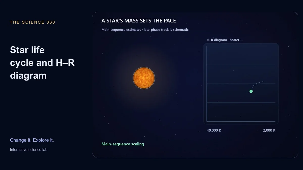
Giving a star more fuel does not necessarily make it live longer. A more massive star can shine so much more intensely that it uses its available fuel faster, ending its main-sequence life much sooner than a faint low-mass star.
The star life cycle simulator compares that tradeoff. Its main-sequence readings are scaling estimates; its later giant and remnant scenes are teaching illustrations. Understanding that boundary makes the tool more useful, not less.
Fuel supply divided by fuel use
A simple lifetime estimate is:
main-sequence lifetime ≈ 10 billion years × (M/M☉)/(L/L☉)
The Sun is the reference: one solar mass and one solar luminosity give 10 billion years. That is an approximate total main-sequence timescale, not the Sun’s remaining lifetime from today.
For another star, you need an estimate of luminosity as well as mass. The lab uses piecewise mass–luminosity relations rather than applying one power law across every mass. Even those relations are broad approximations, not a replacement for a stellar structure calculation.
In the 20-solar-mass preset, the adopted luminosity is 64,000 times solar. The arithmetic gives 10 × 20 / 64,000 Gyr, or about 3.1 million years. The estimate illustrates how rapidly luminosity can overwhelm the advantage of extra fuel.
A red dwarf is a different timescale
At 0.2 solar masses the adopted low-mass relation gives a lifetime near 352 billion years. The exact number should not be treated as a precision forecast, but the comparison is clear: it exceeds the universe’s present age by a large margin.
No such star has yet been observed finishing that entire life. Its late evolution is inferred theoretically. In the playback, those scenes are labeled accordingly rather than presented as a history that astronomers have already watched.
Read the H–R diagram correctly
The horizontal axis places hotter objects to the left. The vertical axis places more luminous objects higher. A large red giant can therefore be cooler at its surface and still be far more luminous than a small hot object.
The main-sequence temperature estimate comes from the luminosity and radius through the Stefan–Boltzmann relation. The later plotted path is schematic, and the playback rail compresses late phases into its final portion. Equal playback steps do not represent equal physical ages across the whole rail.
A remnant is not guaranteed by one slider
The lab uses broad initial-mass branches to illustrate white dwarfs and possible neutron-star or black-hole outcomes. Real outcomes also depend on composition, mass loss, rotation and binary interactions. In particular, the displayed thresholds are not deterministic rules for named stars.
A black hole also has no stellar photosphere in this model. The tool leaves its surface-temperature reading unmodeled instead of assigning an invented glowing stellar surface.
Compare two masses at the same main-sequence playback position, then explain the ratio of their lifetimes. For a different view of compact objects, continue with squeezing a star.
Sources and further reading
 5 amazing physics experiment for your kids
 50 Hilarious Physics Jokes That Will Make You Laugh