How does a star’s mass change its life story?
Initial mass strongly influences a star’s luminosity, fuel-use rate and lifetime. A massive star can die much sooner than a faint low-mass star even though it starts with more fuel.
The main-sequence estimates use simple mass–luminosity and mass–radius scalings. Later phases and the H–R track are explicitly schematic. Scrub the sequence to see the difference between a scale estimate and an illustration of an evolutionary outcome.
Read the companion article for a worked investigation, or continue with squeeze a star.
What to look for
- The one-solar-mass reference gives a main-sequence lifetime of 10 Gyr.
- Brighter stars consume their available fuel faster; fuel supply alone does not set lifetime.
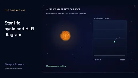
- The H–R diagram places hotter objects to the left and higher luminosities toward the top.
Experiments to try
Load a complete preset, predict what will change, then adjust one control and compare the live measurements.
Sun-like star
Guided experimentThe main-sequence scaling gives one solar luminosity, about 5772 K and a 10-billion-year reference lifetime. Later scenes illustrate expansion and a white dwarf outcome. They are teaching states, not a detailed solar-evolution calculation.
Low-mass red dwarf
Guided experimentA cool, faint star uses fuel slowly. The simple scaling gives a lifetime much longer than the current age of the universe. Its late scenes are theoretical illustrations; we have not observed such a star exhaust its fuel.
Massive star
Guided experimentMore mass supplies more fuel but raises luminosity dramatically. Its estimated main-sequence lifetime is much shorter. A neutron-star outcome here is one possible path; metallicity, mass loss, rotation and binaries can change real remnants.
Compare the cases
| Initial mass | Main-sequence estimate | Late phase in this teaching model |
|---|---|---|
| 0.2 M☉ | About 352 Gyr | Theoretical low-mass evolution |
| 1 M☉ | 10 Gyr | Giant, then white dwarf |
| 20 M☉ | About 3.1 Myr | Supergiant, possible neutron star |
Rounded values and classifications refer to the model and assumptions on this page.
How the model works
Piecewise power laws estimate main-sequence luminosity; radius scales as M^0.8. The Stefan–Boltzmann relation then sets the effective temperature. Lifetime is approximated from mass divided by luminosity.
The first 80% of the playback rail covers the estimated main sequence. The last 20% compresses illustrative giant and remnant states. It is not a uniform physical-time scale; late-phase luminosities and radii are display estimates, not stellar structure solutions.
What the model leaves out
- No nuclear reaction network, stellar structure integration, metallicity, mass loss or binary interactions.
- The initial-mass cuts near 8 and 25 solar masses are illustrative, not deterministic remnant boundaries.
- A black hole has no stellar photosphere; its temperature and luminosity readouts are not modeled.
Common misconceptions
A star is not guaranteed to leave a particular remnant based on initial mass alone. The simplified branches teach broad possibilities and are not predictions for individual named stars.
Frequently asked questions
Is this an accurate prediction for Betelgeuse?
No. Predicting a particular star requires measured properties and a detailed evolution model. This tool is for comparing broad effects of initial mass.
Is the playback rail a linear age axis?
No. Main-sequence time and later illustrative phases are allocated separate portions of the rail so both are visible.
Keep learning
Why massive stars live fast: mass, lifetime and stellar remnants
Estimate main-sequence lifetimes from mass and luminosity, read an H–R diagram, and distinguish schematic evolution paths from detailed stellar predictions.