One hour of astrophotography: why 240 short exposures can differ from six long ones
Sixty minutes of exposure does not always give the same signal-to-noise ratio when you divide it into different numbers of frames. Every readout adds another contribution from detector read noise. Whether that matters depends on how large it is compared with the other noise sources.
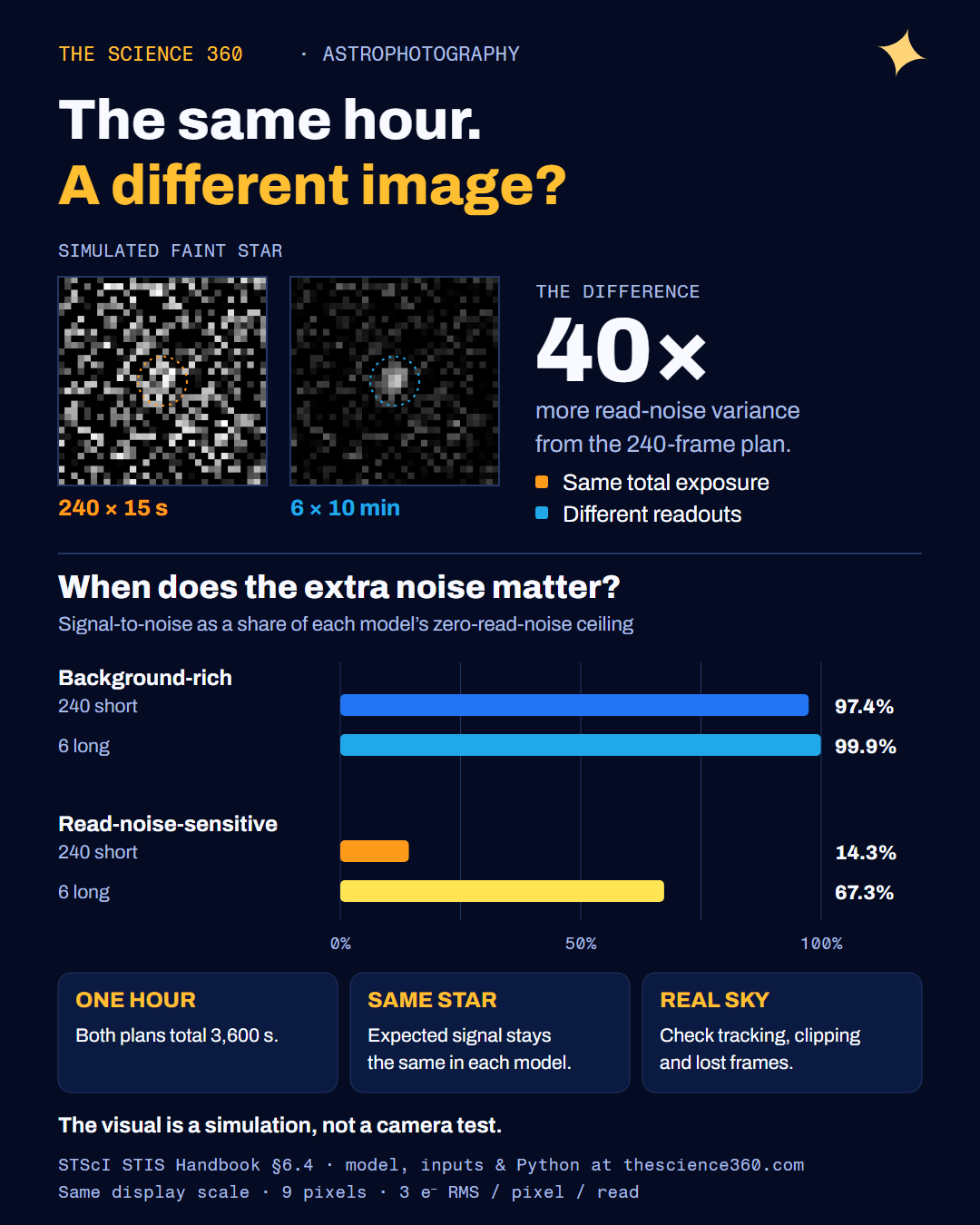
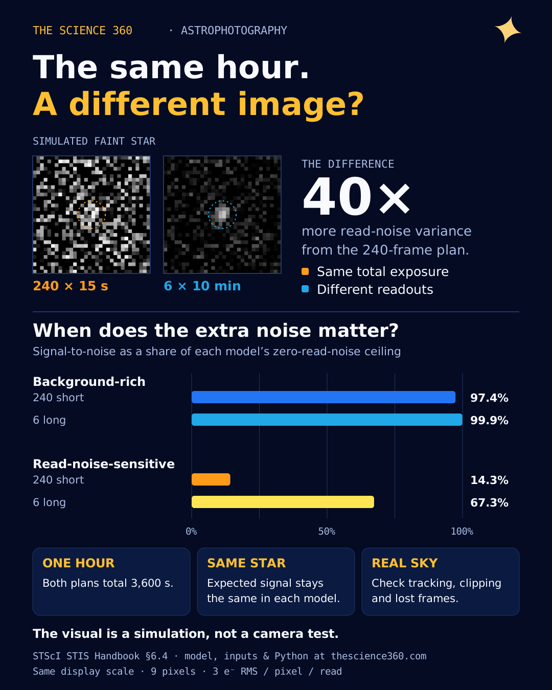
In our illustrative Python model, splitting an hour into 240 fifteen-second frames gives 97.4% of the read-noise-free signal-to-noise ceiling in one regime, but only 14.3% in another. Those are calculated examples with deliberately chosen inputs, not measured camera performance or images of a real target.
The comparison is useful precisely because it holds the total integration time constant. It lets us examine one tradeoff before introducing tracking failures, saturated stars, overheads and all the other reasons an observer might still prefer shorter frames.
What we hold constant
The model follows the source, background, dark-current and read-noise terms in the STScI STIS exposure-time equation. We express everything in electrons, assume no on-chip binning and use a fixed nine-pixel aperture.
For the sum of n equal, independently read exposures:
SNR = S × T / sqrt((S + B + D) × T + n × p × R²)Here S is source signal rate across the aperture, B is sky-background rate across that same aperture, and D is dark-current rate across the aperture, all in electrons per second. T is total integration time in seconds. p is the number of pixels and R is read noise in electrons RMS per pixel per readout.
Our B and D already include the aperture. Multiplying them by nine again would overcount their contribution. The read term still needs the pixel count because R is specified per pixel.
| Assumption | Background-rich illustration | Read-noise-sensitive illustration |
|---|---|---|
| Total integration | 3,600s | 3,600s |
| Aperture pixels | 9 | 9 |
| Read noise per pixel per read | 3e⁻ RMS | 3e⁻ RMS |
| Source rate across aperture | 20e⁻/s | 0.1e⁻/s |
| Sky rate across aperture | 80e⁻/s | 0.01e⁻/s |
| Dark rate across aperture | 0.05e⁻/s | 0.002e⁻/s |
These are two synthetic observing conditions chosen to expose the mechanism. They do not stand for a named camera, filter, sky location or target. We do not use them to rank products.
Same photons expected, different readout budgets
An hour in the first scenario produces an expected 72,000 source electrons regardless of how we split the frames. In the second it produces 360. Longer individual frames do not create additional total integration in this calculation.
What changes is the number of readouts. There are 240 in the fifteen-second case,20 in the three-minute case, and 6 in the ten-minute case. With nine pixels and 3e⁻ RMS read noise, one readout contributes 81e⁻² of variance across the aperture. Two hundred and forty readouts contribute 19,440e⁻²; six contribute 486e⁻².
We add variances, then take a square root. Adding RMS noise values directly would give a different and incorrect model for independent noise contributions.
| Frame plan | Readouts | SNR: background-rich | SNR: read-noise-sensitive |
|---|---|---|---|
| 240 ×15s | 240 | 116.86 | 2.56 |
| 120 ×30s | 120 | 118.38 | 3.58 |
| 60 ×60s | 60 | 119.17 | 4.96 |
| 20 ×180s | 20 | 119.70 | 8.00 |
| 6 ×600s | 6 | 119.89 | 12.07 |
| 1 ×3,600s | 1 | 119.96 | 16.36 |

In the first scenario, source-plus-background Poisson variance is 360,180e⁻². The extra read variance from many short exposures is relatively small. In the second, Poisson variance is only 403.2e⁻². The same readout budget overwhelms that smaller term. That is why identical read noise can have very different practical importance.
A ceiling makes the comparison clearer
Set read noise to zero while keeping the other inputs unchanged. The resulting SNR is 119.97 for the background-rich example and 17.93 for the read-noise-sensitive example. We use these as reference ceilings, not achievable guarantees.
Dividing each calculated SNR by its own ceiling separates the penalty from the scenarios’ very different signal rates. At 180 seconds per frame, one case retains 99.8% of its ceiling; the other retains 44.6%.
You can also derive a planning threshold. Let t be individual exposure duration, so n = T/t. In this idealized model the fractional ceiling becomes:
fraction = 1 / sqrt(1 + p × R² / ((S + B + D) × t))Reaching 95% requires about 7.5 seconds per frame in the first example and 6,694seconds in the second. The latter is longer than our entire one-hour session. It shows that this target fraction is unattainable within the fixed session for the second set of assumptions. It is not a recommendation to take a nearly two-hour frame.
Why an observer might reject the longest exposure anyway
The model has a linear, unsaturated detector and perfect tracking. It loses no frames, has no readout overhead and assumes independent noise after combining frames. Real images need not satisfy those conditions.
STScI’s CCD feasibility discussion explicitly balances read-noise losses against removing cosmic-ray contamination from multiple exposures. Its numerical operating recommendations are for the STIS instrument; copying them into a backyard-camera prescription would be unjustified.
A bright pixel may saturate before a faint target has accumulated much signal. Tracking or guiding can spoil a long frame. Clouds and trails can change which frames are useful. We have not assigned probabilities or numerical losses to these effects. A realistic optimizer would need measurements from the actual equipment and observing conditions.
Background subtraction brings another qualification. Removing the mean sky level does not remove its shot noise. Estimating the background from a finite sample can itself add variance; our simple model assumes that estimate is known well enough to neglect the extra term. Resampling, weighting, clipping and calibration can also alter the noise budget.
The Oxford-hosted introduction to scientific cameras, by Louis Keal of Photometrics, provides additional context on read noise, photon statistics and camera limitations. Its illustrative product examples are not inputs to our calculation.
Reproduce it, then change an assumption
Download the Python script, complete input assumptions and results, CSV and provenance. Run python analyze.py; no external Python packages are needed.
The script checks that every plan totals 3,600 seconds, that SNR stays below the zero-read-noise ceiling and that reducing the number of readouts improves this restricted model. No empirical confidence interval is reported: these are deterministic expected-noise calculations, not fitted observations.
Try reducing R, increasing the background rate or changing the aperture size while keeping the definitions consistent. The result to watch is the relative size of the variance terms. For help understanding the instrument side, see our astronomy-course comparison. The goal is to learn what must be measured before choosing an exposure plan, rather than adopt one duration for every sky.