Double slit experiment explained: interactive simulator • The Science 360

By The Science 360 · Updated October 2026 · 8 min read

What does the double slit experiment show?

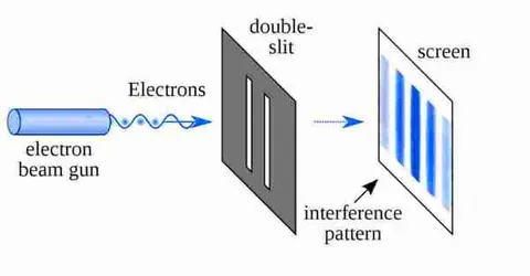
The double slit experiment shows that light, electrons and even large molecules do not travel like tiny bullets: sent through two narrow openings, they build up a pattern of bright and dark stripes on a screen, called interference fringes. The stripes appear even when the particles are sent one at a time, so each particle must be described by a wave that passes both slits. Yet every particle still lands at a single point, and if anything records which slit it used, the stripes vanish. The simulation above lets you change the slit separation and the wavelength, switch between a wave view and single particles, and turn on a which-slit detector.

With the starting settings (slits 0.20 mm apart, light of 550 nm, screen 1.00 m away) the bright fringes are 2.75 mm apart and 13 of them fit under the central hump. For the history, start with Young's double-slit experiment for beginners; for the variations that followed, see variations of the double-slit experiment.

Key results from the simulation

Fringe spacing: bright fringes are λL ÷ d apart. At 550 nm with d = 0.20 mm that is 2.75 mm. Halve d and the spacing doubles.
Colour matters: longer waves spread the fringes. At d = 0.20 mm, red light (650 nm) gives 3.25 mm and violet (420 nm) gives 2.10 mm.
Particles one by one: at 60 per second the first second shows about 60 random-looking dots. After about 1200 dots (twenty seconds) the fringes are clear.
Which-path information: with the detector on, the pattern becomes a single broad hump, half as tall as the fringe peaks. The fringes are gone because the two paths no longer combine.

Six ways to run the experiment

Each section gives the numbers the simulation shows for that setup, and a button that loads it above. The slider is the slit separation d; the buttons also set the wavelength, the view and the detector where the section needs them.

Young’s fringes with waves

d = 0.20 mm, 550 nm

Each slit acts as a new source of waves. At the screen the two waves arrive with a path difference of d sin θ. Where that is a whole number of wavelengths they add (bright); where it is a half-integer they cancel (dark). That gives bright fringes 2.75 mm apart.

The fringes do not run on forever. Each slit is 0.03 mm wide, so its own light spreads into a hump that falls to zero 18.3 mm from the centre. The fringes sit inside that hump, and 13 bright ones fit in it. This hump is the "sinc²" term in the formula.

Fringe gap 2.75 mm Fringes in main peak 13 Hump half-width 18.3 mm Contrast 100%

Slits close together

d = 0.06 mm

Bring the slits to 0.06 mm, only twice the slit width, and the fringes spread to 9.17 mm. Only 3 bright fringes remain under the central hump, which is itself 18.3 mm from the centre to its first dark band.

This is why a school double slit experiment is easier to see with a laser pointer than with a lamp: a close pair of slits gives wide, easy-to-see fringes, but they need light of a single colour so the fringes of different wavelengths do not smear together.

Fringe gap 9.17 mm Fringes in main peak 3 d ÷ slit width 2 Contrast 100%

Slits far apart

d = 0.30 mm

At d = 0.30 mm the fringes tighten to 1.83 mm, and 19 of them crowd under the same hump. With the slits ten slit-widths apart the pattern looks like a fine comb.

Space the slits much further and the fringes become too fine to see by eye, which is one reason atom and molecule experiments need detectors with very small pixels or a magnified image of the pattern.

Fringe gap 1.83 mm Fringes in main peak 19 d ÷ slit width 10 Contrast 100%

Changing colour: red against violet

λ = 650 nm

The fringe spacing is proportional to the wavelength. Red light at 650 nm gives 3.25 mm at d = 0.20 mm, while violet at 420 nm gives 2.10 mm. That is the ratio 650 ÷ 420, about 1.55.

This is also how the experiment can be used to measure the wavelength of light. Measure the fringe gap, the slit separation and the distance to the screen, and λ = d × gap ÷ L. Use the wavelength slider to sweep the spectrum.

Red 650 nm 3.25 mm Green 550 nm 2.75 mm Violet 420 nm 2.10 mm Hump (650 nm) 21.7 mm

One electron or photon at a time

60 particles per second

Switch to particles. Each one lands at a single point, and where it lands is random, but not arbitrary: the chance of landing at a position is proportional to the brightness the wave pattern would have there. The simulation draws every landing position from exactly that distribution, with a fixed random seed so a run repeats.

After a few hundred particles the stripes begin to show. Experiments with single electrons have shown the same slow build-up, with electrons sent so rarely that there is almost never more than one in the apparatus. This is the central mystery: no single dot shows a fringe, yet the crowd does. See the many worlds interpretation for one proposed story, and note that the interpretations all predict the same pattern.

After 1 s 60 dots After 10 s 600 dots After 60 s 3600 dots Fringe gap 2.75 mm

Watching which slit

Which-path information

Turn on "Watch slits" and the fringes disappear. The two single-slit patterns simply add, giving a smooth hump half as tall as the interference peak (equal to the average of the fringes) and 18.3 mm wide to the first zero. The contrast falls from 100% to 0%.

It is the information that does it, not a mind. If something in the apparatus (a photon scattered off the electron, a spin that flips) carries a record of which slit was used, the two paths can no longer combine, whether or not anyone ever reads that record. The popular line that "consciousness collapses the wave" is not what these experiments show. Quantum computers lean on the same principle: they work only while no outside record of the computation leaks, see quantum computing and quantum mechanics.

Contrast 0% Peak height half of fringe peak Hump half-width 18.3 mm Fringes none

Slit separation against fringe spacing

Slit separation d	d ÷ slit width	Gap at 650 nm	Gap at 550 nm	Gap at 420 nm	Fringes in main peak
0.06 mm	2.0	10.8 mm	9.17 mm	7.00 mm	3
0.10 mm	3.3	6.50 mm	5.50 mm	4.20 mm	7
0.15 mm	5.0	4.33 mm	3.67 mm	2.80 mm	9
0.20 mm	6.7	3.25 mm	2.75 mm	2.10 mm	13
0.25 mm	8.3	2.60 mm	2.20 mm	1.68 mm	17
0.30 mm	10.0	2.17 mm	1.83 mm	1.40 mm	19

All values come from the simulation’s formulas for a slit width of 0.030 mm and a screen 1.00 m away, using the small-angle form λL ÷ d for the gap. Real set-ups use different slit widths and distances, but the proportions are the same.

How the simulation works

Light of wavelength λ passes through two slits, each of width a, whose centres are d apart. On a far screen at distance L, a point at height y sees the direction sin θ = y ÷ √(y² + L²). The brightness there is I = I₀ cos²(π d sin θ ÷ λ) × sinc²(π a sin θ ÷ λ), where sinc x = sin x ÷ x. The first factor is the two-slit interference. The second is the single-slit envelope that the fringes sit inside. The simulation uses a = 0.03 mm and L = 1.00 m.

In particle mode the brightness curve is normalised into a probability distribution across the ±25 mm window and the simulation draws 60 landing positions per second from it, using a seeded random number generator. The histogram shows the counts in 120 bins and converges on the curve. With the detector on, the curve is replaced by I = (I₀ ÷ 2) × sinc²(π a sin θ ÷ λ): the sum of the two single-slit patterns with no interference term.

The wave view is a ripple-tank drawing: circular wavefronts from each slit, with the single-slit envelope controlling their strength. To fit the screen, the picture is compressed along the beam so the angles are magnified. The wavefronts keep the same ratios as the real pattern, so the fringe directions in the drawing line up with the graph, but the distances are not the real 1 m. The readings on the graph and on the screen are to scale.

What the model leaves out

Not to scale: a real slit pair is tiny compared with a 1 m screen distance. The drawing exaggerates the angles so you can see the waves.
Far-field only: the formula assumes the screen is far enough away (the Fraunhofer limit). Close to the slits the pattern is more complicated.
One wavelength at a time: white light would show overlapping colour fringes with a white centre. The simulation uses a single wavelength.
Equal slits, perfect coherence: real sources have finite coherence, and unequal slits reduce the contrast. The model uses identical slits and fully coherent light.
The detector is idealised: the toggle represents a perfect which-path record. Partial information gives partially reduced fringes, which the simulation does not show.

Common misconceptions

“The particle changes because a person is looking.” No. A detector (a photon scattering off the particle, say) that stores which-path information is enough. In specially designed "quantum eraser" experiments, erasing the record before it is read can bring the fringes back.

“The electron splits into two pieces.” No. Every detection is a whole electron at one place. The wave describes the probabilities of where it will be found.

“Only quantum objects make interference.” Water waves, sound and light all do. What is surprising is that single particles with mass do the same.

Frequently asked questions

What is the double slit experiment in simple terms?

Shine light or send particles at a barrier with two narrow slits and look at a screen behind it. Instead of two bright lines you see many stripes: interference. It shows that things we think of as particles also behave like waves. A friendly overview is in Young’s double-slit experiment for beginners.

Why does observing the electron change the result?

Because "observing" means interacting with it so that a record of which slit it used exists. With that record, the two paths cannot interfere. Nothing about a conscious observer is required: an automatic detector does it just as well.

What is the formula for the fringe spacing?

Δy = λL ÷ d, where λ is the wavelength, L is the distance from slits to screen and d is the slit separation. With λ = 550 nm, L = 1 m and d = 0.2 mm that is 2.75 mm. It is valid when the angles are small.

Does the electron go through both slits?

The mathematics gives the same pattern whichever way you tell the story. The Copenhagen view says the question has no answer until measured; the many-worlds view says every possibility happens (read about it); pilot-wave theory says each particle takes one path guided by a wave. What everyone agrees on is that detecting the slit removes the fringes.

Has the experiment been done with anything bigger than electrons?

Yes. Interference has been seen with neutrons, atoms, and molecules, including carbon-60 "buckyballs" in 1999 and much larger molecules of about two thousand atoms more recently. Bigger objects have shorter wavelengths, so the fringes are harder to resolve, which is why everyday objects show no interference. More examples are in variations of the double-slit experiment.

Can I do a double slit experiment at home?

A laser pointer and a pair of slits are enough. Scratch two lines about 0.2 mm apart in the blackened coating of a slide, or use a ready-made double-slit card, and shine the laser onto a wall a few metres away. With red light (about 650 nm) and d = 0.2 mm the fringes should be about 3 mm apart for each metre of distance. Never look into the beam.